Dipmeter

	Development Geology Reference Manual
Series	Methods in Exploration
Part	Wireline methods
Chapter	Dipmeters
Author	Joseph F. Goetz
Link	Web page
Store	AAPG Store

As long as oil migrates updip, it would seem there is nothing more fundamental in oil exploration than determining which way is up. It is for this basic purpose that the electric wireline technique known as the dipmeter was designed. From these primitive beginnings, however, the dipmeter has evolved to become a device capable of providing a major input into a complete geological description of the formations crossed by a borehole.

Dipmeter data acquisition

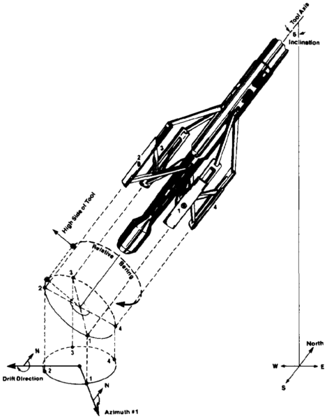
Figure 1 Sketch of a four-arm dipmeter tool illustrating pertinent orientation measurements.
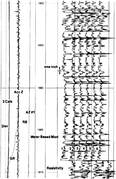
Figure 2 Expanded scale recording of raw dipmeter data from a six-arm tool.

The determination of dip angle and direction of a planar surface requires the elevation and geographical position of at least three points. Dipmeter tools achieve this result by measuring some sensitive formation parameter by means of three or more identical sensors mounted on caliper arms so as to scan in detail different sides of the borehole wall. A bedding plane crossing the borehole at an angle would generate anomalies at each sensor, and these anomalies would be recorded at slightly different depths on the surface recording. The relative displacements and the radial and azimuthal positions of each sensor are then used to compute dip relative to the tool. Microresistivity has been the traditional formation parameter logged. Modern dipmeter tools usually carry more than three sensor arms, the latest version being a device with six arms. More measure points provide the advantage of systematic redundancy, which allows the application of statistical error minimization techniques.

For the results to be geographically significant, it is necessary to define the orientation of the tool in space. This involves continuous measurements of the orientation of the electrode array relative to north, its rotation relative to the high side of the hole, and the inclination of the tool axis from vertical. Such navigation data are produced from the output of an assembly of three orthogonally mounted magnetometers and a similar array of accelerometers. Figure 1 is a sketch of a four-arm tool illustrating the orientation measurements. Figure 2 is an expanded scale recording of the raw dipmeter data showing the orientation curves, calipers, gamma ray, and correlation curves from a six-arm tool. Note that the curves are responding to apparent bedding features less than length::1 in. thick.

Thin bed resolution

Figure 3 Example of thin bed laminated sandstone-shale resolution by means of a dipmeter correlation curve.

In the detailed description of reservoirs, thin bed resolution by wireline techniques is a vital factor. For example, the evaluation of laminated shaly sands can be best accomplished by a sensitive delineation of sand and shale layers. Rather than running a tool designed exclusively for this purpose, money can be saved if the desired information can be derived from a logging tool routinely run for other purposes. Dipmeter surveys, particularly those with a calibrated resistivity scale, can be used for this purpose. Several descriptive properties can be derived from the dipmeter survey:

Lamination thickness and regularity
Layering contrast and frequency
Layering continuity
Flasering and load structures

In Figure 3, a raw dipmeter curve sharply distinguishes between sandstone and shale layers thinner than length::1 in. By establishing a cutoff line as shown, everything to the right can be identified as sand and everything to the left as shale. A reliable measurement of net sand thickness is thus provided, as well as the bulk volume fraction of shale in laminated form for input into laminated shaly sand saturation equations.

Dip computation

The conversion of raw data into useable dip quantities involves three operations:

Curve correlation and displacement definition
Dip determination
Data manipulation and presentation

It is important to realize that each of these stages usually involves filtering to some extent which adds a perspective factor to the results. Therefore, results will vary somewhat with the computation technique employed. The fact is, at any one depth, more than one true dip exists; which dip is reported is a matter of perspective.

In the curve correlation phase, the relative displacement between any set of two curves is determined by using one of many mathematical cross-correlation procedures similar to those used in seismic processing. Usually this involves cross-multiplying the incremental curve values and integrating over some window of depth. The length of the correlation window effectively acts as a stacking filter—the longer the window, the stronger the filtering effect.

In the dip determination phase, one has a choice between a geometric solution and a stochastic approach. While a geometric solution works well in a uniquely determined (three-point) situation, it becomes cumbersome in an overdetermined condition such as that found with four-arm and six-arm tools. In these cases, a stochastic or global mapping approach is more effective in that it uses the redundancy to advantage in minimizing errors. Actually, this approach acts like another stage of stacking filtering. It has the added advantage of neatly solving for orientation of the tool in space.

Dipmeter presentations

Figure 4 Dip data expressed on a standard arrow plot.

The most common presentation of dipmeter data is the arrow or tadpole plot, which is a clever two-dimensional representation of a three-dimensional quantity. In this plot, the base of the arrow is positioned at the depth of the midpoint of the correlation interval, and the distance from the left-hand margin to the base of the arrow is proportional to the true dip angle as calibrated by the scale shown on the heading. The shaft of the arrow points in the downdip direction with true north being straight up the page. Figure 4 is a standard arrow plot that also carries a correlation gamma ray curve and maximum and minimum caliper values. On the right-hand side is a representation of the inclination angle and direction of the tool, which will usually be similar to the deviation of the borehole. A number of other computer generated presentations have been introduced. Many are useful in special situations, but none is a replacement for the arrow plot.

Applications of dipmeters

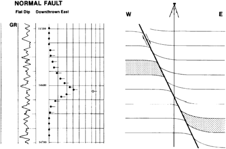
Figure 5 Simple dip model for the description of a normal fault with drag.
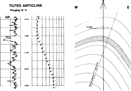
Figure 6 Model of a tilted plunging anticline as it would appear on an arrow plot.
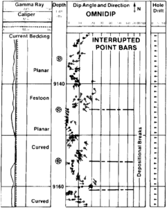
Figure 7 Field example of a detailed dip computation through a sequence of interrupted meandering stream point bars.

Structural applications

Superficially, the determination of structural dip from a dipmeter seems simple and straightforward. In practice, it may be tricky. Difficulties arise from questions of scale and perspective. Structural dip by definition is the dip of recognizable lithological unit boundaries in the general vicinity of the borehole. However, a sharp change in lithology, such as from a shale to a sandstone, is the signature of a catastrophic event in geological history. Therefore, such a contact is liable to be highly irregular over the extremely short section exposed by the borehole. On an outcrop, a field geologist would astutely measure the dip of an eyeball average of the contact. The stringent confines of the borehole offer no such luxury of perspective, and the section of the contact exposed is liable to be highly unrepresentative of the average structural dip. Outcrop perspectives cannot be extrapolated to the borehole, so a different approach is needed.

Because shale is a low energy deposit, it is generally deposited in thin laminations that are parallel, planar, and horizontal at the time of deposition. In the subsurface, then, shale laminations tend to be parallel to one another and parallel to the average of most lithological bed boundaries. In dipmeter computations, there are a number of ways in which the influence of parallel bedding can be accentuated, thus biasing the results toward structural dip. Essentially these are stacking filter effects that can be applied at various stages in the computation chain, such as in the following:

Longer correlation intervals (e.g., 10 ft)
Correlation interval overlap
Global mapping dip computation
Clustering techniques
Polar plots
Vector averaging

Given computation approaches tailored for structural applications, structural dip can then be defined by looking for a consistent trend on the arrow plot. The most repetitive dip should be the structural dip.

The interpretation of structural anomalies is best accomplished by comparison to a set of models—the simpler the model, the better. A simple model, such as the one shown in Figure 5 for a normal fault with drag, is adequate to describe the geometry of such a fault. Figure 6 shows a more complicated arrow plot of low angle dips, reducing to a minimum then increasing to a high angle with the azimuth changing continuously with the dip angle. This is the signature of a tilted plunging anticline. A cross-sectional sketch of the anticline can be produced using the rule of interchangability of perspectives in which the horizontal geometry is interpretable from the vertical pattern of dip. (The application of dipmeter data to solving structural problems is covered in “Evaluating structurally complex reservoirs”.)

Stratigraphic applications

For stratigraphic applications, comparisons to a set of models is also a valid interpretation approach, but in this case, very simple models do not work well. Sedimentary geology is too complex. In fact, hand-drawn models may not be valid at all. It is preferable to use independently verified field examples, such as the one shown in Figure 7. In this example, the sandy sediments are made up of a sequence of interrupted, truncated, and stacked point bars deposited by meandering stream activity. Few complete fining-upward point bar cycles (gravels to sands to shales) are present. Instead, erosional cuts and festoon cross-bedding indicate the start of a new cycle that may or may not be interrupted before the deposition of low angle planar current bedding. (Additional characteristics of meandering streams are covered in Lithofacies and environmental analysis of clastic depositional systems.) In the general case, a catalog of field examples of dip plots from various known depositional environments is a valuable aid to stratigraphic dipmeter interpretation.

Examples of use

Schlumberger, 1986, Dipmeter Interpretation Fundamentals: New York, Schlumberger Ltd., 76 p.
Nurmi, R. D., 1984, Geological evaluation of high resolution dipmeter data: Society of Professional Well Log Analysts' 25th Annual Logging Symposium, vol. 2, paper YY, 24 p.
Sercombe, W. J., B. R. Golob, M. Kamel, J. W. Stewart, G. W. Smith, and J. D. Morse, 1997, Significant structural reinterpretation of the subsalt, giant October field, Gulf of Suez, Egypt, using SCAT, isogon-based section and maps, and 3D seismic: The Leading Edge, vol. 16, p. 1143–1150, DOI: 10.1190/1.1437752.
Hurley, N. F., 1994, Recognition of faults, unconformities, and sequence boundaries using cumulative dip plots: AAPG Bulletin, vol. 78, p. 1173–1185.
Morse, J. D., and C. A. Bengston, 1988, What is wrong with tadpole plots?: AAPG Bulletin, vol. 72, p. 390.
Delhomme, J.-P., T. Pilenko, E. Cheruvier, and R. Cull, 1986, Reservoir applications of dipmeter logs: Society of Petroleum Engineers Paper 15485, 7 p.
Etchecopar, A., J.-L. Bonnetain, 1992, Cross sections from dipmeter data: AAPG Bulletin, vol. 76, p. 621–637.
Bengston, C. A., 1981, Statistical curvature analysis techniques for structural interpretation of dipmeter data: AAPG Bulletin, vol. 65, p. 312–332.
Bengston, C. A., 1982, Structural and stratigraphic uses of dip profiles in petroleum exploration, in Halbouty, M., T., ed., The Deliberate Search for the Subtle Trap: AAPG Memoir 320, p. 619–632.

External links

find literature about
Dipmeter