Multivariate data analysis

Development Geology Reference Manual
Series	Methods in Exploration
Part	Geological methods
Chapter	Multivariate data analysis
Author	K. H. Esbensen, A. G. Journel
Link	Web page
PDF	PDF file (requires access)

Most geological phenomena are multivariate in nature; for example, a porous medium is characterized by a set of interdependent quantities or attributes such as grain size, porosity, permeability, and saturation. Although univariate statistical analysis can characterize the distribution of each attribute separately, an understanding of porous media calls for unraveling the interrelationships among their various attributes. Multivariate statistical analysis proposes to study the joint distribution of all attributes, in which the distribution of any single variable is analyzed as a function of the other attributes distributions.

Multivariate observations are best organized and manipulated as a matrix of sample values, of size (n × P), where n is the number of samples and P is the number of attributes or variables. For example, a (5 × 3) matrix might represent five core samples at different depths on which frequencies of occurrence of three different fossils are recorded. The purposes of multivariate data analysis is to study the relationships among the P attributes, classify the n collected samples into homogeneous groups, and make inferences about the underlying populations from the sample.

As in most statistical endeavors, multivariate data analysis is most efficient if backed by sound prior knowledge (such as geological interpretation) of the underlying phenomenon and a clear idea of project goals. There are many multivariate techniques, and many ways to apply each technique and interpret the results. It is the responsibility of the data analyst (geologist) to formulate the problem context, choose the appropriate multivariate technique, and apply it correctly.

The typical objectives of multivariate data analysis can be divided broadly into three categories.

1. Data description or exploratory data analysis (EDA)--The basic tools of this objective include univariate statistics, such as the mean, variance, and quantiles applied to each variable separately, and the covariance or correlation matrix between any two of the P quantities. Some of the P quantities can be transformed (for example, by taking the logarithm) prior to establishing the correlation matrix. Because the matrix is symmetrical, there are P(P - 1)/2 potentially different correlation values.
2. Data grouping (discrimination and clustering)--Discrimination or classification aim at optimally assigning multivariate data vectors (arrays) into a set of previously defined classes or groups. Clustering, however, aims at defining classes of multivariate similarity and regrouping the initial sample values into these classes. Discrimination is a supervised act of pattern recognition, whereas clustering is an unsupervised act of pattern cognition. Principal component analysis (PCA) allows analysis of the covariance (correlation) matrix with a minimum of statistical assumptions. PCA aims at reducing the dimensionality P of the multivariate data set available by defining a limited number (fewer than P) of linear combinations of these quantities, with each combination reflecting some of the data structures (relationships) implicit in the original covariance matrix.
3. Regression--Regression is the generic term for relating two sets of variables. The first set, usually denoted by y, constitutes the dependent variables(s). It is related linearly to the second set, denoted x, called the independent variable(s). (For details of multiple and multivariate regression analysis, see Correlation and regression analysis.)

A note about outliers

Multivariate data analysis techniques, particularly those relying on some minimization of square deviations, are sensitive to outlying data (values much larger or smaller than the corresponding mean). The data analyst should conduct ample checks for such influence. Once the outliers are detected, they should either be eliminated (if they originated through measurement error) or they should be classified into a separate statistical population. One of the easiest yet most effective ways to detect outliers is to look at the data in some suitable projection section of the multivariate "mathematical space," possibly using some of the techniques described later in this chapter, then iterating the analysis with the outlier-screened subset of the data.

A note about data representativeness

As mentioned in the article on Statistics overview, the available sample data are an incomplete image of the underlying population. Statistical features and relationships seen in the data may not be representative of the characteristics of the underlying population if there are biases in the data. Sources of biases are multiple, from the most obvious measurement biases to imposed spatial clustering. Spatial clustering results from preferential location of data (drilling patterns and core plugs), a prevalent problem in exploration and development. Such preferential selection of data points can severely bias one's image of the reservoir, usually in a nonconservative way. Remedies include defining representative subsets of the data, weighting the data, and careful interpretation of the data analysis results.

Principal component analysis

The main purpose of principal component analysis (PCA) is to identify the most significant variables in a multivariate problem. This is accomplished by reducing the dimensionality of the problem from P, the number of original quantities x₁, ... x_P, to fewer combinations of those quantities, called principal component variables: y₁, ..., y_P0, P₀ ≤ P.

Often, the first few (P₀ < P) first principal components yj may account for a large fraction of the total variablility of the original P variables x_i. The derivation of the principal components does not require any prior assumption on the distribution of the original variables. However, one should usually take care to standardize the measurement units of the x_i's if they correspond to different attribute values. This can be done by dividing each sample value x_i by the standard deviation of all measurements of its type.

Interpretation

A simple examination of these first principal components through their loadings a_ji reveals a great deal about the total variance. If, for example, the first principal component y₁ explains a large proportion of the total variability, its loading factors a_1i relate to the most "influential" variables x_i. These variables in their turn often allow a physical interpretation of y₁. Beware, though, that the ranking of the principal components y_j is based on the variance correlation measure of variability. Alternative measures of variability such as the mean absolute deviation, as well as measures of nonlinear correlation, would lead to different decompositions. Again, the principal components y_j are best interpretd against a prior knowledge (such as geological interpretation) of the underlying phenomenon.

Filtering

The higher components, y_j, j > P₀, usually contain significant "noise," whereas the first (lower) components carry the "signal" information of the initial P variables xi. These higher components can be discarded if they are of no interest. In that case, the multivariate analysis is pursued in the lesser dimensional space of dimension P₀ (there are fewer y's to deal with than original x's). However, in some cases, the noise may be of interest, such as when it represents anomalies in a geochemical data analysis.

The relationship (matrix) defining the principal components y_j can be inverted, yielding the following inverse linear relationship:

$X_{i}=b_{0i}+\sum _{j=1}^{P}b_{ij}Y_{j}$ for all i = 1,...,P

This inverse relationship can be used in estimating (interpolating) a variable x_i from prior estimates of the principal components y_j. The first principal components y_j, j ≤ P₀, can be estimated by some type of regression procedure (such as kriging), while the higher components y_j, j > P₀, corresponding to random noise, can be estimated by their respective means.

Plotting the PCA results

Many plots and scattergrams can be produced using the results of PCA and can be interpreted with the help of prior knowledge about the underlying phenomenon. Such plots may reveal clusters (grouping) or trends in the physical space or the P₀ dimensional space of the first principal components. Interpretation of these clusters and classification of the initial data set (of size n × P) into more homogeneous subsets in the multivariate and/or spatial sense may then be in order. Data analysis can then be pursued within each of these new subsets.

Discriminant analysis (classification)

Figure 1. Plot of two-bivariate distributions, showing overlap between groups a and b along both variables x₁ and x₂. Groups can be distinguished by projecting members of the two groups onto the discriminant function line.

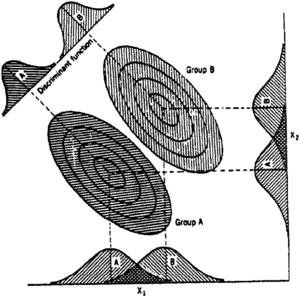
Discriminant analysis (DA) attempts to determine an allocation rule to classify multivariate data vectors into a set of predefined classes, with a minimum probability of misclassification. Consider a set of n samples with P quantities being measured on each. Suppose that the n samples are divided into m classes or groups. Discriminant analysis consists of two steps:

1. The determination of what makes each group different from the others. The answer may be that not all m predefined groups are significantly different from each other.
2. The definition of an allocation rule, usually taking the form of a "score" equal to a particular linear combination of the values of the P quantities.

Using this allocation rule, additional (new) samples can be classified into the predefined groups, and the corresponding probability of misclassification can be estimated (Figure 1).

Discriminant analysis requires the definition of a "distance" between any two groups. A widely used measure is the Mahalanobis distance.

Cluster analysis

The purpose of cluster analysis (CA) is to define classes of samples with multivariate similarity. No prior assumption is needed about either the number of these classes or their structures. Cluster analysis requires and (unfortunately) often depends heavily on a prior choice of a distance measure between any two samples, (x_il, i = 1, ..., P) and (x_il′, i = 1, ..., P). Examples of distances include those represented by the following equations:

Generalized Euclidean distance

$d_{ll'}={\Bigg [}\sum _{i=1}^{P}w_{i}(x_{il}-x_{il'})^{k}{\Bigg ]}^{1/k}$, with k > 0, w_i ≥ 0,

where w_i = weight indicating the relative importance of each variable x_i

Correlation type distance

$d_{ll'}={\frac {\displaystyle \sum _{i=1}^{P}x_{il}x_{il'}}{\sqrt {\displaystyle \sum _{i}x_{il}^{2}\displaystyle \sum _{i}x_{il'}^{2}}}}$

One can also define a distance d_ii′ between any two variables x_i and x_i′ by setting the previous summations over all n samples. Such distances between variables lead to definition of classes of variables having similar sample values. Such classes (clusters) of variables can help defining subsets of the P variables for further studies, with reduced dimensionality.

Figure 2. Dendrogram (by aggregation). Starting from n samples, combine the two most similar samples (here 2 and 3). Then, combine the two nearest groups by either joining two samples or aggregating a third sample to the previous group of two (1 is aggregated to 2 and 3). At the next step, 4 and 5 constitutes a new group, which is then aggregated to the former group (1, 2, 3). The aggregation process stops when there is only one group left. In the last step, group (1, 2, 3, 4, 5) is aggregated to group (6, 7, 8, 9).

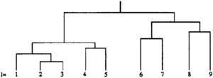
There is a large (and growing) variety of types of cluster analysis techniques:

• Hierarchical techniques provide nested grouping as characterized by a dendrogram (Figure 2).
• Partitioning techniques define a set of mutually exclusive classes.
• Clumping or mixture techniques allow for classes that can overlap.
• Multimode search techniques look for zones in the P-dimensional space having relatively high concentrations of samples.
• Multinormal-related techniques capitalize on a prior hypothesis that each group is P-variate normally distributed.
• Certain other techniques are specific to binary variables.

The problem of preferential sampling in high pay zones, which may lead to more samples having high porosity and saturation values, is particularly critical when performing cluster analysis. If spatial declustering is not done properly before CA, all results can be mere artifacts of that preferential sampling. A related problem is linked to sample locations u_l and u_l′ not being accounted for in the definition of, say, the Euclidean distance between two samples l and l′.

$d_{ll'}={\sqrt {\sum _{i=1}^{P}(x_{il}-x_{il'})^{2}}}$

with x_il = x_i(u_l) and x_il′ = x_i(u_l′) being the two measurements on variable x_i taken at the two locations u_l and u_l′.

In conclusion, although cluster analysis aims at an unsupervised classification, it is best when applied with some supervision and a prior idea of what natural or physical clusters could be. Cluster analysis can then prove to be a remarkable corroboratory tool, allowing prior speculations to be checked and quantified.

See also

• Introduction to geological methods
• Monte Carlo and stochastic simulation methods
• Correlation and regression analysis
• Statistics overview

External links

find literature about Multivariate data analysis

• Original content in Datapages
• PDF file in Datapages

References

- ↑ Everitt, B., 1974, Cluster analysis: London, Heinemann Educational Books Ltd., 122 p.
- ↑ Miller, R. L., and J. S. Kahn, 1962, Statistical analysis in the geological sciences: New York, John Wiley, 481 p.
- ↑ 3.0 3.1 3.2 Davis, J. C., 1986, Statistics and data analysis in geology: New York, John Wiley, 646 p.
- ↑ 4.0 4.1 Hartigan, J. A., 1975, Clustering algorithms: New York, John Wiley, 351 p.
![{\displaystyle d_{ll'}={\Bigg [}\sum _{i=1}^{P}w_{i}(x_{il}-x_{il'})^{k}{\Bigg ]}^{1/k}}](https://wikimedia.org/api/rest_v1/media/math/render/svg/c9097f3c1ddad989f2fcd31d5d9b725ecdc20292)