Standard interpretation

Development Geology Reference Manual
Series	Methods in Exploration
Part	Wireline methods
Chapter	Standard interpretation
Author	Mark Alberty
Link	Web page
Store	AAPG Store

Standard interpretation is the process of determining volumes of hydrocarbons in place from wireline logs, or log interpretation. This process requires four basic steps:

• Determine the volume of shale. Shale affects the response of the various logging devices. To interpret the response for porosity or saturation, the volume of shale must be determined.
• Determine the porosity. Porosity is the fraction of the total rock available for the storage of fluids.
• Determine the formation water resistivity (R_w). The resistivity of the water (without hydrocarbons) is used to interpret the formation resistivity for saturation.
• Determine the water saturation (S_w). A resistivity model is interpreted for saturation. This model relates water saturation, porosity, water resistivity, and volume shale.

Estimation of shale volume

The volume of shale (V_sh) is best estimated by logging measurements that respond primarily to shale, in particular, gamma ray and spontaneous potential (SP). The most common methods for estimating shale volumes from gamma ray and SP logs are outlined here. Other measurements can be used under special conditions to estimate shale volumes, such as the resistivity in very high resistivity formations, the compensated neutron in very low porosity formations, or density versus neutron crossplots in known lithologies.

Shale volume from gamma ray

Figure 1 Nonlinear shale volume chart. Copyright: Western Atlas International, 1985; courtesy of Atlas Wireline Services Division of Western Atlas International, Inc.

Application

The gamma ray can be an excellent estimator of shale volume in areas with little uranium and where radioactive salts are associated primarily with clay minerals.

Method

The two most frequently used methods of estimating shale volume from the gamma ray log are the linear and the nonlinear estimators. Both methods require determining the gamma ray response (GR) at the depth of interest and determining the response associated with a clean reservoir having no shale (GR_cl) and a zone of 100% shale (GR_sh).

The linear method is the simplest, but it tends to overestimate shale in the intermediate ranges of shale volumes. The linear response equation is

$V_{\rm {sh}}={\frac {{\mbox{GR}}_{\rm {sh}}-{\mbox{GR}}}{{\mbox{GR}}_{\rm {sh}}-{\mbox{GR}}_{\rm {cl}}}}$

The nonlinear method begins by estimating the shale volume from the linear equation and then correcting that estimation using a chart as shown in Figure 1. First, one marks the horizontal axis (labeled “radioactivity index”) with the linear estimation of shale volume. One then proceeds vertically to the appropriate rocks and then horizontally to read the corrected volume of shale.

Advantages

The gamma ray method is very simple, fast, and generally the most reliable. It can be used with the potassium or thorium curves and with the uranium corrected total gamma ray curve from the spectral gamma ray.

Limitations

Gamma ray readings must be corrected for hole size first. This method does not work well in areas where radioactivity is not primarily associated with the clays, such as in feldspathic sands.

Shale volume from spontaneous potential (SP)

Application

The SP can be an fair estimator of shale volume in areas where mud filtrate and formation water resistivities contrast.

Method

The estimation of volume shale from the SP requires determining the SP response at the depth of interest and determining the response associated with a clean reservoir with no shale (SP_cl) and a zone of 100% shale (SP_sh). The response equation is

$V_{\rm {sh}}={\frac {{\mbox{SP}}_{\rm {sh}}-{\mbox{SP}}}{{\mbox{SP}}_{\rm {sh}}-{\mbox{SP}}_{\rm {cl}}}}$

Advantages

The SP method is very simple and fast.

Limitations

This method does not have good vertical resolution. It overestimates shale volume in hydrocarbon-bearing zones, and it is ensitive to the selection of clean reservoir and shale points. It will not work in zones where R_w ≈ R_mf or in oil-based muds.

Porosity estimation

Any logging device primarily affected by the presence of porosity can be used to estimate porosity (ϕ). Best results are generally produced by the density, compensated neutron, and sonic logs. When using a single porosity measuring device such as the density, neutron, or sonic, assumptions are normally required to estimate porosity. These assumptions are the lithology and the fluid properties, which must be determined from local knowledge. If multiple porosity measuring devices are recorded, the multiple measurements can frequently be used together to determine porosity and lithology. (Determination of lithology is discussed in Quick-look lithology from logs.)

Porosity from density

Application

Density is a good method for determining either total or effective porosity in single or multiple mineral, fluid-filled reservoirs. It is extremely useful in combination with core measurements of grain density.

Method

The method of estimating porosity from the density requires determining the matrix density (ρ_ma), the density log reading (ρ_b), and the fluid density (ρ_fl at the depth of interest. The matrix density is determined by the lithology. Normally, sandstone is 2.65 g/cm³, limestone is 2.71 g/cm³, and dolomite is 2.87 g/cm³. The fluid density is dependent upon the salinity of water and the density of hydrocarbon. Freshwater has a density of 1.0 g/cm³ and saltwater approximately 1.1 g/cm³. Hydrocarbon density can vary widely from 0.05 g/cm³ for gas at low pressures to nearly 1.0 g/cm³ for certain oils. A typical value for oil is 0.8 g/cm³.

The density response equation is

$\phi _{\rm {D}}={\frac {\rho _{\rm {ma}}-\rho _{\rm {b}}}{\rho _{\rm {ma}}-\rho _{\rm {fl}}}}$

Advantages

This method can be used to determine porosity accurately when matrix and fluid densities are known. It can be used to determine either total or effective porosity through the selection of appropriate matrix density. Matrix density can be accurately determined from core measurements. Linear volumetric response allows expansion for multiple mineral formations.

Limitations

The shallow investigation of the density normally results in investigating the flushed zone; one must typically use flush zone fluid properties in its interpretation. This method is difficult to use accurately in gas reservoirs due to the difficulty of determining the appropriate fluid density of the flushed zone. One should use apparent matrix and fluid densities adjusted to the relationship of the ratio of twice the atomic number divided by the atomic weight (2Z/A) for freshwater-filled limestone. This method only investigates one side of the borehole (typically the low side).

Porosity from compensated neutron

Application

The compensated neutron measurement gives a rough estimate of the total porosity in simple fluid-filled reservoirs. It is very sensitive to gas, and consequently, it is useful as a gas indicator in conjunction with the density measurement. It can also be used with density to determine both lithology and porosity in non-gas bearing zones. It is sensitive to clay content.

Method

The compensated neutron measurement is recorded at the wellsite to provide the correct water-filled porosity in a user-specified matrix, normally limestone or sandstone. If recorded on the appropriate matrix, the log values can be corrected for environmental effects and then used as an estimate of water-filled porosity. If the zone of interest contains fluids with lower hydrogen indexes than water, the porosity will be underestimated.

Advantages

A very strong response to gas is useful in identifying gas reservoirs (indicates low porosity) when used in conjunction with density or sonic porosity measurements. A neutron and density combination is very useful in identifying mineralogy. The most practical porosity measurement is through the casing.

Limitations

Since shallow investigation normally results in investigating the flushed zone, one must typically use flush zone fluid properties in interpretation. This method investigates omnidirectionally around the borehole and typically requires considerable environmental corrections. It is sensitive to standoff from the borehole wall and needs effective decentralization for reasonably accurate results.

Porosity from sonic

Application

The compressional sonic log can be used as a moderately good estimator of porosity in water and, to some degree, oil-filled rocks.

Method

The two most frequently used methods of estimating porosity from sonic measurements are the Wyllie time average method and the Raymer-Hunt-Gardner field observation method. Both methods require determining the sonic response (Δt₁) at the depth of interest and determining the response associated with the matrix (Δt_ma). Typical values for Δt_ma are 55.5 μsec/ft for sandstone, 47.5 μsec/ft for limestone, and 43.5 μsec/ft for dolomite. (A more complete listing of interval traveltimes for common minerals is given in the chapter on Difficult lithologies in Part 4.)

The Wyllie time average method requires an estimate of fluid interval transit time (Δt_fl). Typical values range from 189 μsec/ft for saltwater to 204 μsec/ft for freshwater. This method tends to overestimate porosity in uncompacted sandstones and hydrocarbon-bearing reservoirs. Empirical corrections to lessen this error can be implemented using the compaction factor (Cp) and hydrocarbon correction (Hy) terms. Cp describes the influence of pore pressure on the sonic porosity equation. It is normally estimated from comparison of density and apparent sonic porosity or from the sonic response in nearby shale (Cp = Δt_sh/100.0). Hy is approximate and is set equal to 0.9 for oil and 0.7 for gas. The Wyllie time average equation is

$\phi _{\rm {s}}={\frac {\Delta t_{\rm {l}}-\Delta t_{\rm {ma}}}{\Delta t_{\rm {fl}}-\Delta t_{\rm {ma}}}}{\frac {\mbox{Hy}}{\mbox{Cp}}}$

The Raymer-Hunt-Gardner equation is an empirical approach developed from a statistical analysis of a database of sonic measurements and independently determined porosity. This equation is

$\phi _{\rm {s}}=C{\frac {\Delta t_{\rm {l}}-\Delta t_{\rm {ma}}}{\Delta t_{\rm {l}}}}$

The value of C can vary between 0.625 and 0.70, depending upon local conditions. The most widely accepted value is 0.67. A value of 0.60 is recommended for gas reservoirs.

Graphical charts for solving these equations are normally in service company chartbooks.

Advantages

The sonic method is very fast and can be very accurate when parameters are tuned to a particular reservoir. For this reason, the sonic porosity method is commonly used in the appraisal of field development wells.

Limitations

The interpretation of sonic logs is sensitive to formation pressure and rock compressibility, particularly in unconsolidated rocks. Results are variable in hydrocarbon-bearing zones due to the uncertainty of the appropriate C or Δt_fl for hydrocarbons. The sonic log may measure the interval traveltime of the flushed zone or of the unaltered formation depending upon the depth of invasion and the relative velocities of the two zones. This can produce some uncertainty in selection of appropriate interpretation parameters.

Porosity from density and neutron

Figure 2 Density-neutron crossplot chart. Copyright: Schlumberger Well Services, 1979.

Uses

Porosity and lithology can both be determined from simultaneous use of both the density and neutron measurements. (These methodologies are discussed further in Quick-look lithology from logs and Difficult lithologies.) Two primary methods are used.

Method 1

The first method requires determining the lithology that will cause both the density and neutron response equations to produce similar porosity values. One of the easiest methods is to solve these two equations simultaneously in a graphical manner. Service companies provides their customers with chartbooks containing density versus neutron crossplots for their particular tools. An example is shown in Figure 2. First, one should mark the horizontal axis with the environmentally corrected neutron reading in limestone porosity units and the vertical axis with the bulk density. Be sure that the chart and neutron log are on compatible lithology scales (limestone). The point where the two meet represents the porosity and lithology of a clean, water-filled rock. The porosity is determined by interpolating between equal porosity lines connecting the common porosity points on the sandstone, limestone, and dolomite lines. The lithology is determined by interpolating between the labeled lithologies.

Advantages

The density-neutron generally provides the best sensitivity to lithology, porosity, hydrocarbons, and shaliness.

Limitations

Results are degraded in rugose holes where the density is unable to maintain proper wall contact. In heterogeneous formations, the density may respond to formation characteristics occurring on only one side of the hole while the neutron responds to the formation on all sides. In additional, the two devices have different depths of investigation. These conditions may lead to inappropriate conclusions concerning lithology and/or porosity.

Note

Other crossplot techniques available are the density-sonic and the density-neutron. The density-sonic is inappropriate for fractured formations and generally has poor sensitivity to lithology. The neutron-sonic has reduced sensitivity to lithology compared to the density-neutron, but it has increased sensitivity to the presence of gas. Both of these techniques are subject to the limitations of measuring porosity with the sonic discussed earlier.

Method 2

An approximation of the crossplot answer for clean reservoirs can be made using the following equation:

$\phi ={\sqrt {\frac {\phi _{\rm {N}}^{2}+\phi _{\rm {D}}^{2}}{2}}}$

where

• ϕ = estimated porosity
• ϕ_N = neutron porosity for the appropriate lithology
• ϕ_D = density porosity for the appropriate lithology

Advantages

This method provides quick, reasonable answers even in the presence of gas.

Limitations

This method requires that the porosities be determined for the appropriate lithology. It is only an approximate answer (typically within one or two porosity units). Accuracy decreases with increasing shale content and gas effects.

Determination of water saturation

Water saturation (S_w) is most often determined from the logging measurement of resistivity and knowledge of porosity, water resistivity, and shale volume. The interpretation procedures can be divided into two separate procedures—one for shaly and one for clean reservoirs.

Water saturation in clean reservoirs

Application

The Archie equation is the primary method for interpreting resistivity measurements. Either the induction or the laterolog wireline measurement can be used for formation water saturation in areas where the formation water contains moderate to saturated amounts of dissolved salts and the reservoir rock contains no shale or clay.

Method

The predominant electrical conductor in subsurface formations is salt water. Most other fluids and minerals normally encountered in reservoirs are nonconductors. The analysis of the actual conductivity (or resistivity) of the rock compared to the conductivity (or resistivity) of the same rock when fully saturated with water serves as the basis for determining water saturation from wireline logs. This fundamental relationship was described by Gus Archie and is expressed by the following equation:

$S_{\rm {w}}^{n}={\frac {F\times R_{\rm {w}}}{R_{\rm {t}}}}$

where

• S_w = water saturation
• F = formation resistivity factor
• R_w = resistivity of formation waters
• R_t = true formation resistivity
• n = saturation exponent

The formation resistivity factor, F, describes the tortuosity of the conductivity paths (pore space) in the rock. It can be determined in the laboratory from cores or it can be estimated from the following relationship:

$F={\frac {a}{\phi ^{m}}}$

where ϕ is the porosity of the rock and a and m are determined from local experience. The most common values for a and m are as follows:

In soft formations: a = 0.81, m = 2.0, or a = 0.62, m = 2.15

In hard formations: a = 1.0, m = 2.0

In fractured rocks, m tends toward lower values, and in vugular rocks, it tends toward higher values.

The value of the resistivity of the formation waters, R_w, can be determined from the SP in water sands, from the Archie equation applied to nearby water sands, from water samples, or from local experience (see “Deterrnination of Water Resistivity”). This value of the true resistivity of the formation, R_t, can be determined from analysis of the dual induction or dual laterolog measurements (see “Preprocessing of Logging Data”).

The saturation exponent, n, describes how the tortuosity of the conductive paths in the formation increases as the water saturation decreases. The value of n can be determined in the laboratory from measurements on cores or from local experience. The most typically used value for n is 2.0.

Advantages

This method is the simplest for interpreting saturation in clean sands. It can be calibrated with cores for increased accuracy.

Limitations

It only works for clean reservoirs. The value for m is very difficult to determine accurately in fractured or vugular reservoirs.

Water saturation in shaly reservoirs

Application

Many variations on the Archie equation have been developed over the years to describe the influence of clay or shale as a conductor in reservoir rocks. These methods simply have an additional clay or shale term included to the basic Archie equation to account for the clay conductivity. Variations of the different equations have arisen to handle the different distributions that shale or clay may take in the rock. (For references that provide guidelines for selecting the appropriate equation for a particular formation, see Difficult lithologies.)

Method

The Simandoux equation is a good general purpose equation that accounts for the influence of shale with regard to water saturation. The Simandoux equation is

${\frac {1}{R_{\rm {t}}}}={\frac {S_{\rm {w}}^{2}}{F\times R_{\rm {w}}{\big (}1-V_{\rm {SH}}{\big )}}}+{\frac {V_{\rm {SH}}\times S_{\rm {w}}}{R_{\rm {SH}}}}$

where

• S_w = water saturation
• F = formation resistivity factor
• R_sH = resistivity of shale
• V_SH = volume of shale
• R_w = resistivity of formation waters
• R_t = true formation resistivity
• n = saturation exponent

The selection of parameters is similar to that described for clean reservoirs. Note that the equation is quadratic, making it significantly more difficult to solve manually for saturation. Normally, saturations in shaly sands are determined using computers or programmable calculators.

Advantages

This method accounts for shale conductivity in reservoir rocks. Different equations exist for structural, laminated (interbedded), dispersed, and intermixed distribution clays and shales.

Limitations

One must understand the shale distribution to select the appropriate equation. The value of m is very difficult to determine accurately in fractured or vugular reservoirs. In low salinity reservoirs, these equations overestimate water saturation due to a phenomenon called excess clay conductivity; in these cases, a different model (such as dual water or Waxman-Smit) may be more appropriate.

Example interpretation

• 

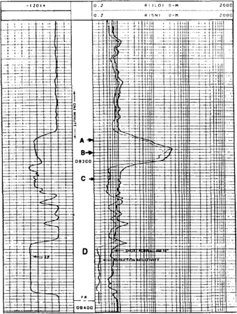
  Figure 3 Induction log for example interpretation.

• 

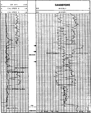
  Figure 4 Density-neutron log for example interpretation.

The logs in Figures 3 and 4 are used for this example. Figure 3 is a deep induction log recorded with a shallow resistivity device and SP, while Figure 4 is a compensated density-neutron log with a gamma ray. The well is an unconsolidated sand and shale sequence from the Gulf Coast area. Interval D is apparently wet because of the low resistivity. R_w can be determined in this interval from either the SP or by the Archie method (see Determination of water resistivity). R_w was determined here by the Archie method to be 0.026 Q-m at formation temperature. For the purposes of this example, no environmental corrections were made and were assumed to be unnecessary.

Point A is above the gas-oil contact, as indicated by the severe crossover of the density and neutron porosities that were recorded on a sandstone matrix. The density-porosity log reads 35% and the neutron log 11%. Thus, we have

$\phi ={\sqrt {\frac {\phi _{\rm {N}}^{2}+\phi _{\rm {D}}^{2}}{2}}}={\sqrt {\frac {0.11^{2}+0.35^{2}}{2}}}$

$\phi _{\rm {A}}=0.26,{\mbox{ or }}26\%$

Point B is in a light oil column as indicated by the slight crossover of the density and neutron porosities that were recorded on a sandstone matrix. The density log reads 30% and the neutron log 17%. Thus,

$\phi ={\sqrt {\frac {\phi _{\rm {N}}^{2}+\phi _{\rm {D}}^{2}}{2}}}={\sqrt {\frac {0.17^{2}+0.30^{2}}{2}}}$

$\phi _{\rm {B}}=0.24,{\mbox{ or }}24\%$

Point C is also apparently in a light oil column as indicated by the slight crossover of the density and neutron porosities that were recorded on a sandstone matrix. The density log reads 31% and the neutron log 23%. Thus,

$\phi ={\sqrt {\frac {\phi _{\rm {N}}^{2}+\phi _{\rm {D}}^{2}}{2}}}={\sqrt {\frac {0.23^{2}+0.31^{2}}{2}}}$

$\phi _{\rm {C}}=0.27,{\mbox{ or }}27\%$

The formation resistivity factor can be calculated from these porosities using one of the relationships for soft formations:

$F_{\rm {A}}={\frac {0.81}{\phi ^{2}}}={\frac {0.81}{0.26^{2}}}=12.0$

$F_{\rm {B}}={\frac {0.81}{\phi ^{2}}}={\frac {0.81}{0.24^{2}}}=14.1$

$F_{\rm {C}}={\frac {0.81}{\phi ^{2}}}={\frac {0.81}{0.27^{2}}}=11.1$

Saturations can be estimated from the Archie equation since there is little or no volume shale, as indicated by the gamma ray. R_t should be determined after environmental corrections, but is assumed here to be equal to the deep induction resistivity (R_ILd) due to the high porosity and relatively shallow mvasion. In zone A, R_t is 5.0 Ω-m, in zone B, 13 Ω-m, and in zone C, 0.55 Ω-m.

Assuming n to be 2.0, Archie's equation can be written and solved for each zone as follows:

$S_{\rm {wA}}={\sqrt {\frac {F\times R_{\rm {w}}}{R_{\rm {t}}}}}={\sqrt {\frac {12.0\cdot 0.026}{5.0}}}=0.25$

$S_{\rm {wB}}={\sqrt {\frac {F\times R_{\rm {w}}}{R_{\rm {t}}}}}={\sqrt {\frac {14.1\cdot 0.026}{13.0}}}=0.17$

$S_{\rm {wC}}={\sqrt {\frac {F\times R_{\rm {w}}}{R_{\rm {t}}}}}={\sqrt {\frac {11.1\cdot 0.026}{0.55}}}=0.72,{\mbox{ or }}72\%$

This analysis found zone A to be a gas-bearing sand with 26% porosity and 25% water saturation. However, water saturation is most likely overestimated due to the proximity of the massive conductive shale bed. Zone B was found to be a light oil sand with 24% porosity and 17% water saturation. Zone C was found to be a residual light oil sand with 27% porosity and 72% water saturation.

See also

• Basic tool table
• Basic open hole tools
• Basic cased hole tools
• Difficult lithologies
• Determination of water resistivity
• Preprocessing of logging data
• Quick-look lithology from logs

External links

find literature about Standard interpretation

• Original content in Datapages
• Find the book in the AAPG Store