Seismic data: two- or three-dimensional interpretation

Exploring for Oil and Gas Traps
Series	Treatise in Petroleum Geology
Part	Predicting the occurrence of oil and gas traps
Chapter	Interpreting 3-D seismic data
Author	Geoffrey A. Dorn
Link	Web page
Store	AAPG Store

Three-dimensional seismic interpretation is not just dense 2-D seismic interpretation. Although it is certainly possible to interpret the 3-D seismic volume as a dense 2-D grid (in fact, some early interactive interpretation systems actually encouraged this), this is neither an effective nor an efficient approach to the interpretation. The results are generally of poorer quality and require significantly more effort than interpreting the data in a 3-D fashion.

Figure 1 Opaque volume from a 3-D seismic survey in the southern North Sea Gas Basin. From Dorn. Courtesy SEG.

Volume visualization

Volume visualization provides an effective tool for data preview. We can view animations of opaque slices through the data volume along any orientation, and we can control the slicing interactively. We can also control the opacity of the volume. By making the data volume partially transparent, we can see the structure of strong reflections prior to doing any interpretation. It may also be possible to isolate elements of depositional systems by controlling the color and opacity mappings.

Data preview example

Figure 1 is an opaque volume from a 3-D seismic survey in the southern North Sea Gas Basin. Four horizons are indicated: Top Chalk, Top Keuper, Top Zechstein, and Top Rotliegend. By visualizing the volume with the opacity set so that only the strongest peaks and troughs are opaque, we can see the overall 3-D structure of these horizons prior to interpretation (Figure 1b).

Examining Figure 1b, we can note that the anticline at the Top Chalk has a different trend than the anticline at the Top Keuper. Some faulting is evident along the north end of the Top Keuper horizon extending roughly parallel to the trend of the anticline. The Top Zechstein and Top Keuper are approximately conformable in this volume, and the strong amplitude reflections from the west are dipping. Top Rotliegend fault blocks are also evident. By using motion (e.g., rotation around the time axis) and stereo displays, the structures, their relationships, and the positions of specific reflections become much more obvious than they are in the still images in Figure 1.

The 2-D approach

Two-dimensional interpretation of a 3-D seismic volume involves limiting your views of the data, and your interpretation, to lines and cross-lines. Typically, this approach to interpretation has its roots in two things. First, the interpreter is comfortable with seismic sections. Second, the interpreter new to 3-D interpretation may simply decide that “there is too much data to possibly look at all of it.” Two-dimensional interpretation of the 3-D volume results in loss of information and is the least efficient approach to interpreting the data. Modern interactive systems provide a variety of tools that allow interpreters to perform the interpretation in a more 3-D fashion.

Never enough data

The first rule of 3-D seismic interpretation is that there is never enough data. The problem we are trying to solve with seismic interpretation is always underdetermined. There is never enough information to uniquely define the geology of the subsurface in the area of the 3-D survey. In some instances, you may decide to disregard some of the data collected. If you do not use it all, then you are reducing resolution and control.

Weaknesses of vertical sections

A second rule for 3-D seismic interpretation is that the survey is always oriented at 45° to the trend of faults, channels, and other features of interest. There will always be faults or channels oriented at angles between 0° and 45° relative to the orientation of the vertical section you are interpreting. If you only look at vertical sections, you will always miss important features of the geology.

Example of seeing faults

Figure 1 Images from a 3-D survey in the Gulf of Mexico. From Dorn. Courtesy SEG.

Figure 1 shows several images from a 3-D survey in the Gulf of Mexico. Figure 1a is a dip magnitude map at an interpreted horizon in the data, showing several steep dip (pink) lineaments associated with normal faults that cut the horizon. Arrows b, c, and d show the orientation and direction of three traverses cut through the volume at angles of approximately 90°, 45°, and 10° to the trace of the fault in the center of the horizon. Figure 1b, c, and d are traverses b, c, and d, respectively. The fault is clearly interpretable in the centers of the traverses that cut the fault at angles of 90° and 45°. However, it would be very difficult to interpret the fault on Figure 1d, the oblique traverse. This geometric effect produces a blind zone on vertical sections that are oriented between +/–20° of the trend of a fault. As a result, if you are only interpreting vertical seismic sections, you will fail to see faults that have trends in this zone. The same phenomenon occurs with depositional stratigraphy.

The best section to image a channel is a section oriented at 90° to the trend of the channel.

Start with time slices

The first step toward 3-D interpretation of a 3-D volume is to use time slices. The value of time-slice interpretation for faults is fairly obvious. Regardless of the strike of the fault, most fault surfaces intersect the time slice at an angle between 45° and 90° to the plane of the time slice

Computer limitations

• 

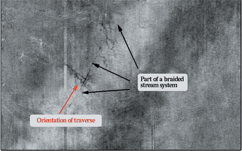
  Figure 2 Time slice from a 3-D survey in the North Sea. From Dorn. Courtesy SEG.

• 

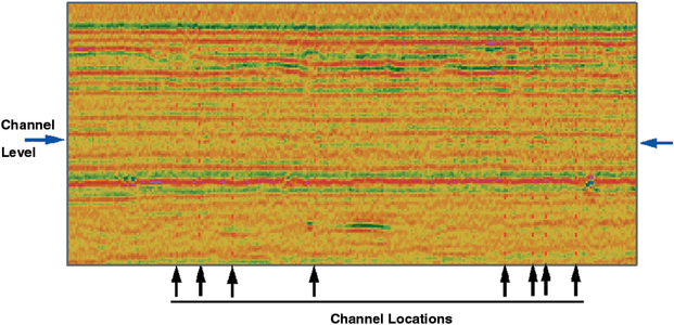
  Figure 3 Traverse cut through the data in a direction perpendicular to the channel system. From Dorn. Courtesy SEG.

Depositional systems are typically more interpretable on time slices than they are on vertical sections. Figure 2 is a time slice from a 3-D survey in the North Sea. Aportion of a braided stream system is clearly evident.

Figure 3 is a traverse cut through the data in a direction perpendicular to the channel system. Horizontal arrows indicate when the channel system occurs, and vertical arrows show the location of each of a number of individual channels cut by the traverse. It is safe to say that most if not all of these channels would have been missed if the interpretation had been limited to vertical sections.

See also

• Seismic data
• Data preview
• Picking horizons in 3-D data
• Surface slicing

External links

find literature about Seismic data: two- or three-dimensional interpretation

• Original content in Datapages
• Find the book in the AAPG Store

References

- ↑ 1.0 1.1 1.2 1.3 Dorn, G. A., 1988, Modern 3-D seismic interpretation: The Leading Edge, v. 17, no. 9, p. 1262-1272. Cite error: Invalid
<ref>tag; name "Dorn_1998" defined multiple times with different content