Well log analysis for reservoir characterization

Wiki Write-Off Entry
Student Chapter	Universitas Gadjah Mada
Competition	December 2014

Well log is one of the most fundamental methods for reservoir characterization, in oil and gas industry, it is an essential method for geoscientist to acquire more knowledge about the condition below the surface by using physical properties of rocks. This method is very useful to detect hydrocarbon bearing zone, calculate the hydrocarbon volume, and many others. Some approaches are needed to characterize reservoir, by using well log data, the user may be able to calculate:

1. shale volume (Vsh)
2. water saturation (Sw)
3. porosity (φ)
4. permeability (k)
5. elasticity (σ, AI, SI, etc.)
6. reflectivity coefficient (R)
7. other data that the user need

The interpretation of well log data must be done in several steps and it is not recommended for the user to analyze them randomly because, the result might be a total error. Figure 1 shows the steps for reservoir characterization by using well log data. Basically, there are two types of properties that will be used in reservoir characterization, they are petrophysics (shale volume, water saturation, permeability, etc.) which are more geology-like and rock physics (elasticity, wave velocity, etc.) which are more geophysics-like. Every properties are related each other, the relation between each properties is shown in figure 2, the author called it as the “fish diagram”. There are many techniques to find a hydrocarbon bearing zone, the user may use RHOB-NPHI cross over (with some corrections), reflectivity coefficient (just like in seismic interpretation), AI anomaly, etc. Every method has their own weaknesses, so it is a wise decision to use every method to acquire the right result. There are so many kinds of modern logs, see table 1 for the information about the logs and also their uses.

Table 1 The functions of every log in petrophysical and rock physics properties calculation and analysis.

Name	Uses
Gamma Ray (GR)	Lithology interpretation, shale volume calculation, calculate clay volume, permeability calculation, porosity calculation, wave velocity calculation, etc.
Spontaneous Potential (SP)	Lithology interpretation, Rw and Rwe calculation, detect permeable zone, etc.
Caliper (CALI)	Detect permeable zone, locate a bad hole
Shallow Resistivity (LLS and ILD)	Lithology interpretation, finding hydrocarbon bearing zone, calculate water saturation, etc.
Deep Resistivity (LLD and ILD)	Lithology interpretation, finding hydrocarbon bearing zone, calculate water saturation, etc.
Density (RHOB)	Lithology interpretation, finding hydrocarbon bearing zone, porosity calculation, rock physics properties (AI, SI, σ, etc.) calculation, etc.
Neutron Porosity (NPHI)	Finding hydrocarbon bearing zone, porosity calculation, etc.
Sonic (DT)	Porosity calculation, wave velocity calculation, rock physics properties (AI, SI, σ, etc.) calculation, etc.
Photoelectric (PEF)	Mineral determination (for lithology interpretation) *not used in this article

• 

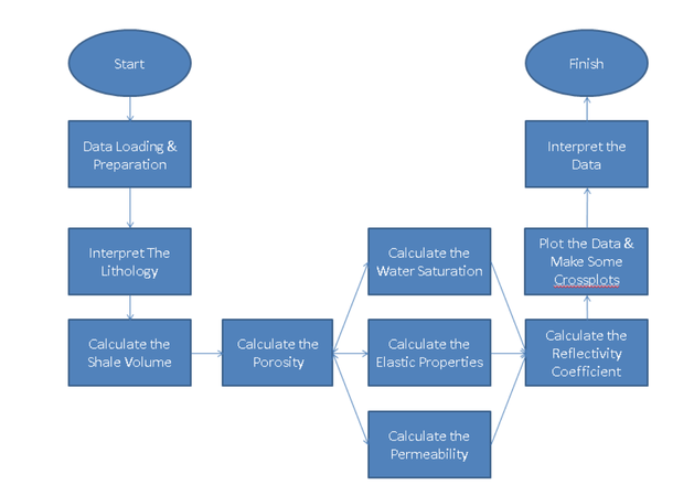
  Figure 1-Flowchart to analyze well logs that must be done to characterize an oil or gas reservoir, the user should follow these steps in order to acquire the correct result.

• 

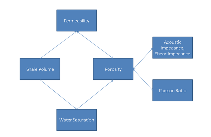
  Figure 2-Fish diagram that shows the relation between petrophysical and elasticity properties.

Interpret the Lithology

Figure 3-The use of gamma ray log to determine the lithology.

The user will be able to interpret the lithology by using several logs, there are gamma ray, spontaneous potential, resistivity, and density log. Basically, a formation with high gamma ray reading indicates that it is a shaly or shale, when the low gamma ray reading indicates a clean formation (sand, carbonate, evaporite, etc.), lithology interpretation is very important in reservoir characterization because, if the lithology interpretation is already wrong, the other steps such as porosity and water saturation calculation will be a total mess.

Calculate the Shale Volume

This second step could be done by using gamma ray log, Larionov (1969) proposed two formulas to calculate the shale volume, those formulas are:

Larionov (1969) for tertiary rocks:

${\text{Vsh}}=0.083(23.7\times {\text{IGR}}-1)$

Larionov (1969) for older rocks:

${\text{Vsh}}=0.33(22\times {\text{IGR}}-1)$

${\text{IGR}}={\frac {GRlog-GRmin}{GRmax-GRmin}}$

where IGR is the gamma ray index, Vsh is the shale volume, GRlog is the gamma ray reading, GRmax is the maximum gamma ray reading, and GRmin is the minimum gamma ray reading. Calculating shale volume is an important thing to do because, it can be useful to calculate the water saturation, if the reservoir has shale within its body (shaly) such as in delta, that reservoir may has higher water saturation because, shale has the ability to bound together with water which will increase the water saturation. Shale volume could also be used as an indicator of zone of interest or not, many users usually will not classify a formation with high shale volume as a reservoir because of its low permeability.

Calculate the Porosity

Porosity is the void or space inside the rock, they are very useful to store fluids such as oil, gas, and water, they are also able to transmit those fluids to a place with lower pressure (probably surface) if they are permeable (see permeability in section 5). Porosity calculation is the third step of well log analysis and it could only be done correctly if the first step (lithology interpretation) is correct. There are many methods that can be used to calculate the porosity, the user may use density log, sonic log, neutron log, or combination between them, but the most common one is neutron-density log combination. The user may use the formulas below to calculate the neutron-density porosity:

$\Phi {\text{nd}}={\frac {{\mathit {\Phi }}d+{\mathit {\Phi }}n}{2}}$

for non-gas reservoir, or

$\Phi {\text{nd}}={\sqrt {\frac {{\mathit {\Phi }}d^{2}+{\mathit {\Phi }}n^{2}}{2}}}$

for gas reservoir

φd value:

$\Phi {\text{d}}={\frac {\rho matrix-\rho log}{\rho matrix-\rho fluid}}$

 where ρmatrix is the matrix density (the value depends on the lithology, see table 2 for the value reference), ρfluid is the fluid density (see table 2 for the value reference), ρlog is the density log reading, φd is the density-derived porosity, φn is the neutron porosity (from neutron log reading), and φnd is the neutron-density porosity. If the lithology interpretation has been wrong from the start, the density-derived porosity will also show the wrong result which means that the neutron-density porosity will also be wrong, so the ability to interpret the lithology correctly is an important asset for the user.

Table 2-Matrix density and fluid density reference table (Halliburton, 1991) with some additions.

Lithology	Value (gr/cm3)	Fluid	Value (gr/cm3)
Sandstone	2.644	Fresh Water	1.0
Limestone	2.710	Salt Water	1.15
Dolomite	2.877	Methane	0.423
Anhydrite	2.960	Oil	0.8
Salt	2.040

Calculate the Water Saturation

There are so many methods to calculate water saturation, the user may use Archie’s, Simandoux’s (1963), etc. which will use different formula for every one of them, but in this article, the author will use Simandoux’s (1963) method, to calculate the water saturation by using this method, the user will need to use the following formula:

${\frac {1}{Rt}}={\frac {Sw^{2}}{F\times Rw}}+{\frac {Vsh\times Sw}{Rsh}}$

${\displaystyle {\text{Rw}}={\frac {Rwe+0.131\times 10\left({\frac {1}{\log \left({\frac {$BHT}{19.9}}\right)}}\right)^{-2}}{-0.5\times Rwe+10\left({\frac {0.0426}{\log \left({\frac {BHT}{50.8}}\right)}}\right)}}}

${\displaystyle {\text{Rwe}}=Rmf\times 10^{\frac {SP}{61+0.133\times$BHT}}}

${\text{F}}={\frac {a}{{\mathit {\Phi }}^{m}}}$

where Rt is the true resistivity of the formation (deep resistivity), Rw is the formation water resistivity, Vsh is the shale volume, Rsh is the resistivity of shale, Rwe is the formation water  resistivity (without thermal effect), BHT is the bottom hole temperature, Rmf is the mud filtrate resistivity, SP is the spontaneous potential log reading, F is the formation volume factor, a is the tortuosity factor, m is the cementation exponent, φ is the porosity, and Sw is the water saturation. To acquire the value of a and m, the user will need to create a pickett plot, but according to Asquith, the reference value is shown in table 3. 

Table 3. Tortuosity factor (a) and cementation exponent (m) reference table.

Lithology	a (tortuosity factor)	m (cementation exponent)
Carbonate	1.0	2.0
Consolidated Sandstone	0.81	2.0
Unconsolidated Sandstone	0.62	2.15
Average Sand	1.45	1.54
Shaly Sand	1.65	1.33
Calcareous Sand	1.45	1.70
Carbonate (Carothers, 1986)	0.85	2.14
Pliocene Sand	2.45	1.08
Miocene Sand	1.97	1.29
Clean, granular formation	1.0	φ(2.05-φ)

Calculate the Permeability

Defined as the rock’s ability to transmit fluid, higher permeability shows that the rock is able to transmit fluid easiliy and it means that the more hydrocarbon that can be produced daily, it is affected by many factors, such as shale volume, effective porosity, and many other else. There are so many methods that can be used to calculate the permeability, but in this article, the author will use Coates’s (1981) method, the formula is listed below:

${\text{k}}=100\times {\frac {{\mathit {\Phi }}^{2}\times (1-Swirr)}{Swirr}}$

where k is the permeability, φ is the porosity, and Swirr is the irreducible water saturation (the author use 0.3 as the assumption for this variable). From the formula above, we can conclude that if the irreducible water saturation is at 1, then the permeability will be zero.

Calculate the Elasticity

There are so many kinds of elastic properties of a rock, there are Acoustic Impedance (AI), Shear Impedance (SI), Poisson Ratio (σ), etc. and most of them depend on the wave velocity and density.

$AI=\rho \times V\rho$

$SI=\rho \times Vs$

$\sigma ={\frac {\left({\frac {Vp}{Vs}}\right)^{2}-1}{2\left({\frac {Vp}{Vs}}\right)^{2}-1}}$

where Vp is the P-Wave velocity and Vs is the S-Wave velocity. According to Castagna et al, Vp and Vs can be calculated by using this formula:

$Vp(km/s)=5.81-9.42\times {\mathit {\Phi }}s-2.21\times Vclay$

$Vp(ft/s)=(5.81-9.42\times {\mathit {\Phi }}s-2.21\times Vclay)\times 300$

$Vs(km/s)=3.89-7.07\times {\mathit {\Phi }}s-2.04\times Vclay$

$\Phi {\text{s}}={\frac {\Delta tlog-\Delta tmatrix}{\Delta tfluid-\Delta tmatrix}}$

${\text{Vclay}}={\frac {0.5\times Vsh}{1.5-Vsh}}$

where φs is the sonic-derived porosity, Vclay is the clay volume, Δtlog is the sonic log reading (DT), Δtmatrix is the matrix transit time (see table 4 for reference value), and Δtfluid is the fluid transit time (see table 4 for reference value). Theoretically, a formation with high density will has lower transit time (Δtlog) which will cause the seismic wave to travel faster in that formation. An anomaly in density and sonic log (Δt) in a formation may indicates the presence of fluids in that formation (see section 9). 

 Table 4. Matrix and fluid transit time reference table.

Lithology	Value (μs/ft)	Fluid	Value (μs/ft)
Consolidated Sandstone	55.5	Fresh Water	218
Unconsolidated Sandstone	51.5	Salt Water	189
Limestone	47.5	Oil	238
Dolomite	43.5	Methane	626
Anhydrite	50.0
Gypsum	52.0
Salt	67.0

Reflectivity Coefficient

The reflectivity coefficient could be derived from density and sonic log then the user may complete this method simply by using the AI difference between every formation which shows the reflectivity coefficient (R) which shows the rock’s ability to reflect the seismic wave to the surface, the formula is listed below:

${\text{R}}={\frac {\rho 2\times Vp2-\rho 1\times Vp1}{\rho 2\times Vp2+\rho 1\times Vp1}}={\frac {AI2-AI1}{AI2+AI1}}$

where ρ1 is the density of the rock in the first formation, ρ2 is the density of the rock in the second formation, Vp1 is the P-Wave velocity in the first formation, and Vp2 is the P-Wave velocity in the second formation. The reflectivity coefficient is very related with seismic, it represents how good is the rock’s ability to reflect seismic wave, if the reflectivity is high, then more seismic wave will be reflected back to the surface which will be shown by the presence of bright spot, but if the reflectivity is very low, it is called dim spot, both of them could be used as hydrocarbon indicator.

Case Study

Data

The author used the well data from South Barrow 18’s well (downloaded from http://energy.cr.usgs.gov/OF00-200/WELLS/SBAR18/LAS/SB18.LAS), the data are shown in figure 4A.

Lithology Interpretation

By using gamma ray (GR), spontaneous potential (SP), resistivity (LLD and LLS), and density log (RHOB), the user will able to interpret the lithology (figure 5A), there are 4 lithology in this well, they are sandstone, shaly sandstone, sandy shale, and shale. There is also a bad hole here (figure 4B), shown by the caliper log’s value that is very big which indicates a heavily weathered layer, the user should not try to interpret or analyze logs in a bad hole, because the well data may contain error which is caused by the inability of the instruments to reach the formation, so instead of measuring the formation’s properties, they are measuring the empty zone so the data cannot be trusted anymore.

By using gamma ray log (see figure 3), the user will be able to differentiate the shale (or shaly) or non-shale formation. With the help of spontaneous potential log, the user could give some corrections to the gamma ray log, shale usually has positive SP log reading, when clean (sand, etc.) formation has very negative SP log reading, shaly formation lies between them (not too negative). Resistivity log will also help the user to differentiate the lithology, sandstone or carbonates have high resistivity, the average resistivity value in this well is around 8 Ωm, because of that, formation with higher resistivity than that can be classified as sandstone (if the gamma ray value is low to medium) or carbonates (if the gamma ray value is very low). The last one is the density log (RHOB), with this log, the user could differentiate if the formation is tight or not, also with this log, the user could differentiate between shale-shaly-non shale formation, shale usually has low density when non-shale formation usually has density higher than shale, shaly formation lies between them, if the formation has a very high density log reading, the user may classify that formation as a “tight” formation, when its gamma ray log reading is around 30-50, we may call it as a “tight sandstone” formation, or if the gamma ray log reading is very log (usually below 15 API), the resistivity and density log reading is very high, it could be an anhydrite which is a good cap rock in petroleum system. Table 5 shows the characteristics of some rocks that can be used to differentiate the lithology, but please remember that the reference value is relatively different for every well, so the user should not confused with this issue. 

Table 5. Petrophysical properties reference of some sedimentary rocks.

Lithology	Gamma Ray (API)	Spontaneous Potential (mV)	Resistivity (Ωm) [If shale resistivity is 8]	Density (gr/cm3)
Sandstone	30 – 50	Varies, very negative	10+	2.4 – 2.8
Shaly-sandstone	50 – 75	Varies, negative	8 < Resistivity < 10	Around 2.4
Sandy-shale	75 – 90	Varies, negative	Around 8	Around 2.3
Shale	Higher than 90	Higher than 0	8	Around 2.3
Anhydrite	Below 15	-	Very high, up to 100+	Up to 2.9
Coal	Varies	-	Varies	Varies, could be 1.7 – 2.2
Crystalline	Below 30	-	Very high, up to 150+	Up to 2.9
Limestone	20 – 30	-	Very high, up to 100+	2.3 – 2.7

Petrophysical & Rock Physics Properties Analysis

Based on the formulas in section 2-6, the author has done some calculations about the well log data (see figure 6 and 7), from figure 6, we can see the petrophysical properties (Vshale, Sw, φ, and k) and from figure 7 we can see the rock physics properties (AI, SI, Vp/Vs, and σ). Based on the data, we can see that the reservoirs in this well (see figure 9A or B) have low shale volume content (compare figure 9A or 9B with figure 6), which indicates that those reservoirs should have higher permeability than the other formations, those reservoirs are also have low water saturation (see figure 6) which indicates a high amount of hydrocarbon proven by the velocity ratio vs AI crossplot (figure 11) and if we correlate it with the porosity, we can conclude that those reservoirs have good porosity and low water saturation which make them good reservoirs with high hydrocarbon content.

To look for reservoir by using rock physics method, the user can do it by making a crossplot between the Depth vs AI (figure 10A and 10B), theoretically, the AI of every rock should increase as it deposited in a deeper place, and by quick looking into the anomaly, the user can say that it is a zone of interest but some corrections with the other data must be done to get the more accurate result. From figure 8 we can observe the reflectivity coefficient which mainly talks about density and wave velocity of every formation, the user may use them as hydrocarbon detector, the formation with very negative and very positive R value shows that there is a very big density and wave velocity difference between the upper and lower formation which can be used to detect hydrocarbon (direct hydrocarbon indicator), after that, we should do some correction by using gamma ray, resistivity, and caliper log (figure 9A), the user should also has the knowledge about the bit size, the blue line in figure 9A shows that not every very negative or very positive R value represents dim spot or bright spot, caliper log and bit size data shows that there is a bad hole there so that the R value in 1930-1960ft is not a dim spot or bright spot, but it is just an error which is caused by the bad hole, but the other direct hydrocarbon indicator (2050-2080ft) is an oil reservoir (reservoir A) and the other reservoir (reservoir B) which lies from 2120ft is a gas reservoir, both of them are sandstone reservoirs (see figure 5B).

Based from petrophysics point of view, a reservoir usually has lower density than the same lithology that surrounds the reservoir, low gamma ray, and high resistivity response (figure 9B). First, the density, a formation with low density usually has high porosity which is needed to store the hydrocarbon fluid. Second, the gamma ray response, the usual reservoir are sandstone, carbonates, or shaly-sandstone, a formation with very high gamma ray response usually contains more shale than the one with low gamma ray response, shale will block the interconnected pores which will reduce the effective porosity and permeability and that will prevent the hydrocarbon fluid to be stored inside the pores. The last one is resistivity, oil and gas has higher resistivity than water, so by looking onto the well log data, a zone of interest (where cross over between RHOB-NPHI is present) is not always a reservoir if the resistivity is low.

• 

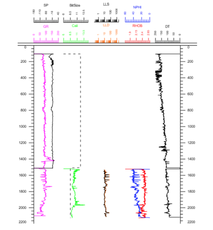
  Figure 4A-Well logs that will be used for the interpretation of South Barrow 18 well.

• 

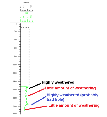
  Figure 4B-Determining a bad hole based on bit size and caliper log response.

• 

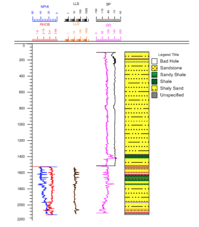
  Figure 5A-Lithology interpretation of South Barrow 18 well, the author use the combination of GR-SP- Resistivity-RHOB logs to interpret the lithology (NPHI log is present here to aid the author in locating a hydrocarbon bearing zone.

• 

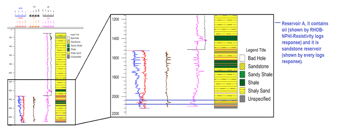
  Figure 5B-Reservoir A (upper) lithology interpretation.

• 

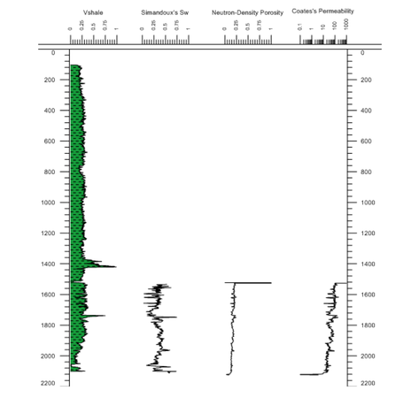
  Figure 6-The calculation result of Vshale, Sw, φ, and k in South Barrow 18 well.

• 

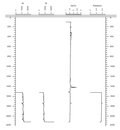
  Figure 7-The calculation result of AI, SI, Vp/Vs, and σ in South Barrow 18 well.

• 

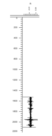
  Figure 8-The result of reflectivity coefficient calculation, a very high or very low R value is usually caused by the presence of hydrocarbon or big difference of density and wave velocity between two formations.

• 

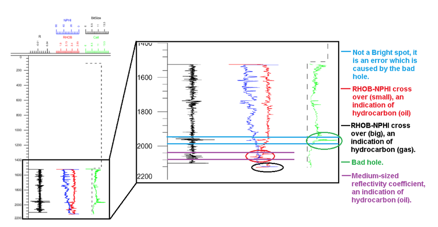
  Figure 9A-The relation between log data and reflectivity coefficient, from this figure, we can see that the detection zone of interest (red and black circle) can also be done by looking onto the R, a formation that contains hydrocarbon usually has very low or very high R (purple lines).

• 

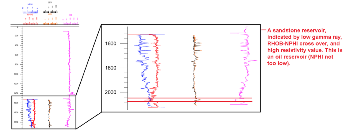
  Figure 9B-The technique to detect hydrocarbon bearing zone by using RHOB-NPHI, resistivity, and gamma ray log.

• 

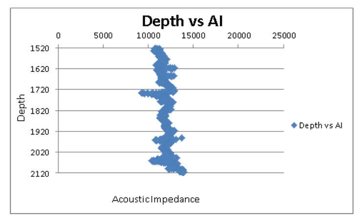
  Figure 10A-Crossplot between depth and acoustic impedance (AI).

• 

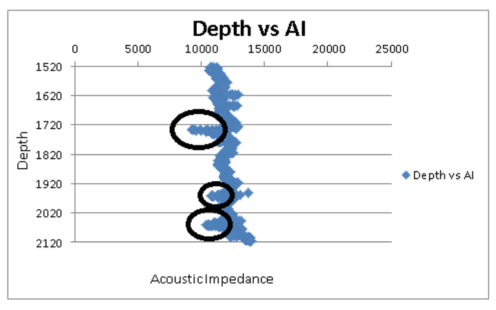
  Figure 10B-Crossplot between depth and acoustic impedance (AI), the black circles show the acoustic impedance anomaly.

• 

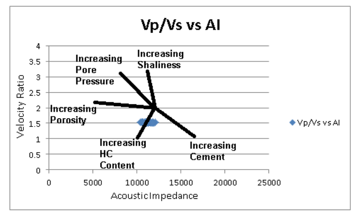
  Figure 11-Crossplot between velocity ratio (Vp/Vs) and acoustic impedance (AI), by using this crossplot, we can determine the formation orientation whether it contains hydrocarbon or not, how about the pressure, etc.

Sources

• Ijasan, O., C. Torres-Verdín, and W. E. Preeg, 2013, Interpretation of porosity and fluid constituents from well logs using an interactive neutron-density matrix scale: Interpretation, v.1, no. 2, p. T143-T155.
• Tiab, D., and E. C. Donaldson, 2011, Petrophysics: Theory and practice of measuring reservoir rock and fluid transport properties: Gulf Professional Publishing.
• Jorgensen, D. G., 1989, Using geophysical logs to estimate porosity, water resistivity, and intrinsic permeability.
• Doveton, J. H., 1986, Log analysis of subsurface geology: Concepts and computer methods.
• Ellis, D. V., and J. M. Singer, 2007, Well logging for earth scientists (Vol. 692). Dordrecht: Springer.
• Muammar, R., 2014, Application of Fluid Mechanics to Determine Oil and Gas Reservoir’s Petrophysical Properties By Using Well Log Data.
• Balan, B., S. Mohaghegh, and S. Ameri, 1995, State-of-the-art in permeability determination from well log data: part 1-A comparative study, model development: SPE paper 30978, p. 17-21.

bottom hole temperature

American Petroleum Institute