Uploads by Importer
Jump to navigation
Jump to search
This special page shows all uploaded files.
| Date | Name | Thumbnail | Size | Description | Versions |
|---|---|---|---|---|---|
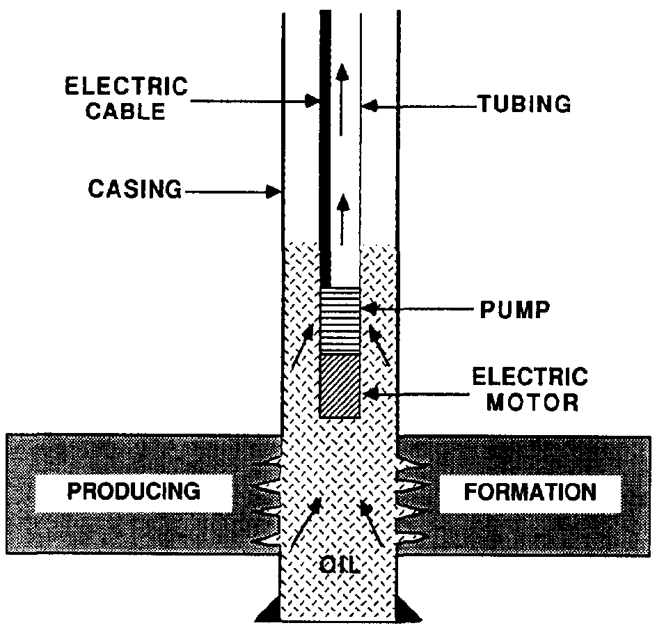
| 17:24, 13 January 2014 | Artificial-lift fig1.png (file) |  |
27 KB | {{copyright|AAPG}} Electric submersible pump. (From <xref ref-type="bibr" rid="pt09r5">Conoco Inc., 1990</xref>.) Category:Production engineering methods | 1 |
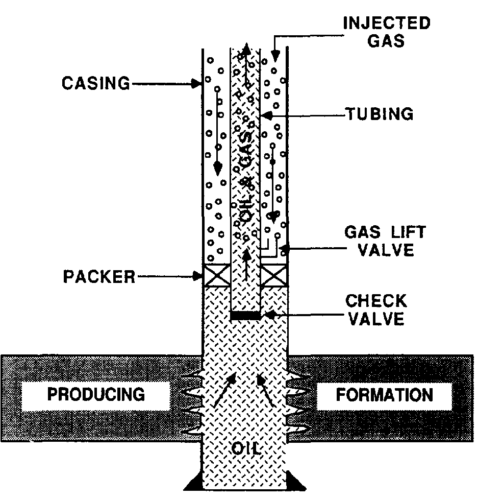
| 17:24, 13 January 2014 | Artificial-lift fig2.png (file) |  |
29 KB | {{copyright|AAPG}} Gas lift system. (From <xref ref-type="bibr" rid="pt09r5">Conoco Inc., 1990</xref>.) Category:Production engineering methods | 1 |
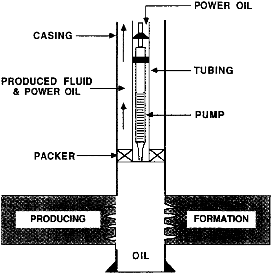
| 17:24, 13 January 2014 | Artificial-lift fig3.png (file) |  |
52 KB | {{copyright|AAPG}} Hydraulic piston pump. (From <xref ref-type="bibr" rid="pt09r5">Conoco Inc., 1990</xref>.) Category:Production engineering methods | 1 |
| 17:24, 13 January 2014 | Artificial-lift fig4.png (file) |  |
93 KB | {{copyright|AAPG}} Beam pumping system. (From <xref ref-type="bibr" rid="pt09r5">Conoco Inc., 1990</xref>.) Category:Production engineering methods | 1 |
| 17:49, 13 January 2014 | Full-waveform-acoustic-logging fig1.png (file) |  |
19 KB | {{copyright|AAPG}} FWAL microseismograms recorded (a) at two source-receiver separations and (b) In a “soft” formation at two source-receiver separations. Category:Geophysical methods | 1 |
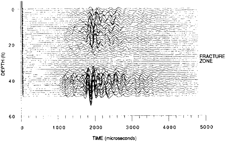
| 17:49, 13 January 2014 | Full-waveform-acoustic-logging fig2.png (file) |  |
66 KB | {{copyright|AAPG}} FWAL microseismograms across a fracture zone. Category:Geophysical methods | 1 |
| 17:49, 13 January 2014 | Full-waveform-acoustic-logging fig3.png (file) |  |
12 KB | {{copyright|AAPG}} Plot of the difference between the measured slowness and the predicted elastic slowness (ΔΔT) against the core measured permeability values for both the limestone-dolomite and the sand-shale examples. (After Burns et al., 1988.) ... | 1 |
| 18:14, 13 January 2014 | Basic-cased-hole-tools fig1.png (file) |  |
70 KB | {{copyright|Schlumberger, 1986}} Typical presentation of a pulsed neutron log. Copyright: Schlumberger, 1986. Category:Wireline methods | 1 |
| 18:21, 13 January 2014 | Basic-open-hole-tools fig1.png (file) |  |
78 KB | {{copyright|Schlumberger, 1983}} A typical log showing SP, gamma ray, dual Induction, and sonic measurements. Copyright: Schlumberger, 1983. Category:Wireline methods | 1 |
| 18:21, 13 January 2014 | Basic-open-hole-tools fig2.png (file) |  |
71 KB | {{copyright|Schlumberger, 1983}} A typical log showing density, compensated neutron, Pe, gamma ray, and caliper measurements. Copyright: Schlumberger, 1983. Category:Wireline methods | 1 |
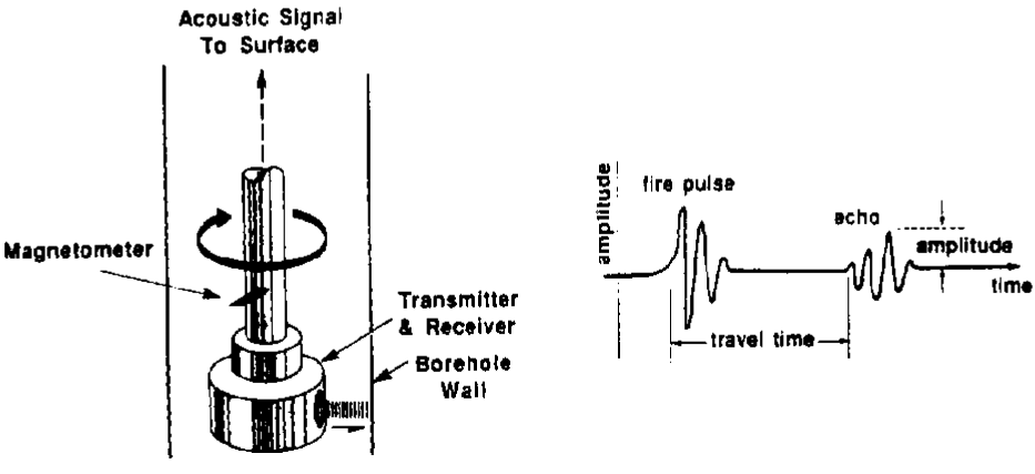
| 18:53, 13 January 2014 | Borehole-imaging-devices fig1.png (file) |  |
21 KB | Borehole televiewer technique. (From Zemanek et al., 1969.) Category:Wireline methods | 1 |
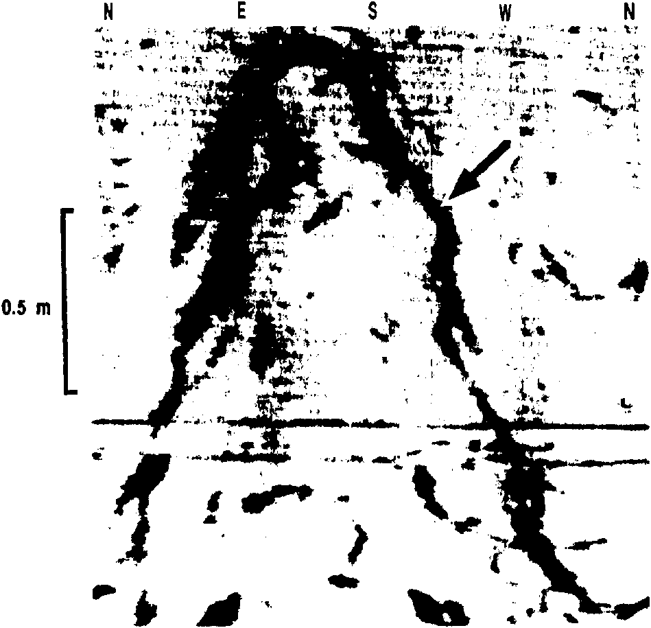
| 18:53, 13 January 2014 | Borehole-imaging-devices fig2.png (file) |  |
576 KB | Drill marks (arrow) on borehole televiewer images. Category:Wireline methods | 1 |
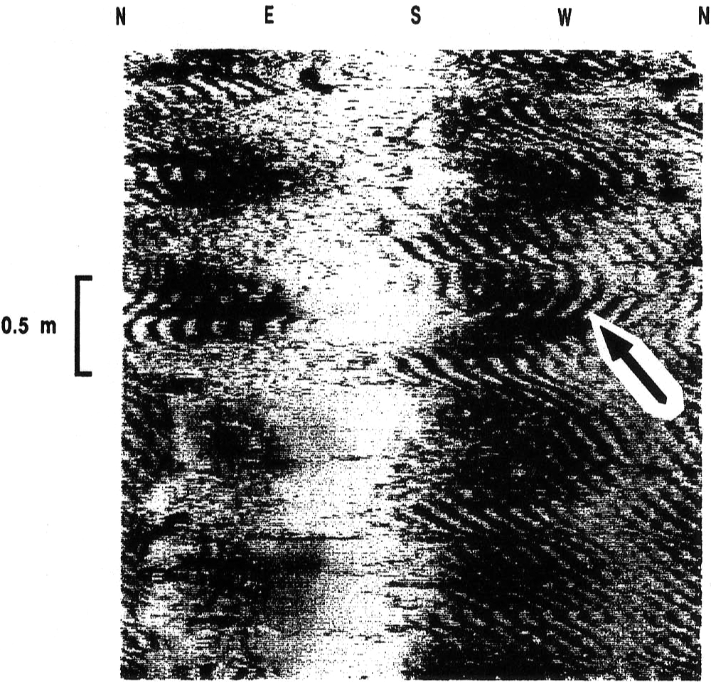
| 18:53, 13 January 2014 | Borehole-imaging-devices fig3.png (file) |  |
25 KB | Borehole televiewer Image showing fracture (arrow) crossing the wellbore. Category:Wireline methods | 1 |
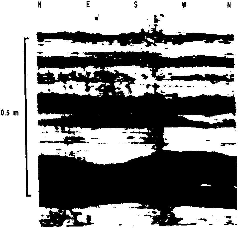
| 18:53, 13 January 2014 | Borehole-imaging-devices fig4.png (file) |  |
16 KB | Borehole televiewer images showing shale layers (dark) intercalated with limestone layers (bright). Category:Wireline methods | 1 |
| 18:53, 13 January 2014 | Borehole-imaging-devices fig5.png (file) |  |
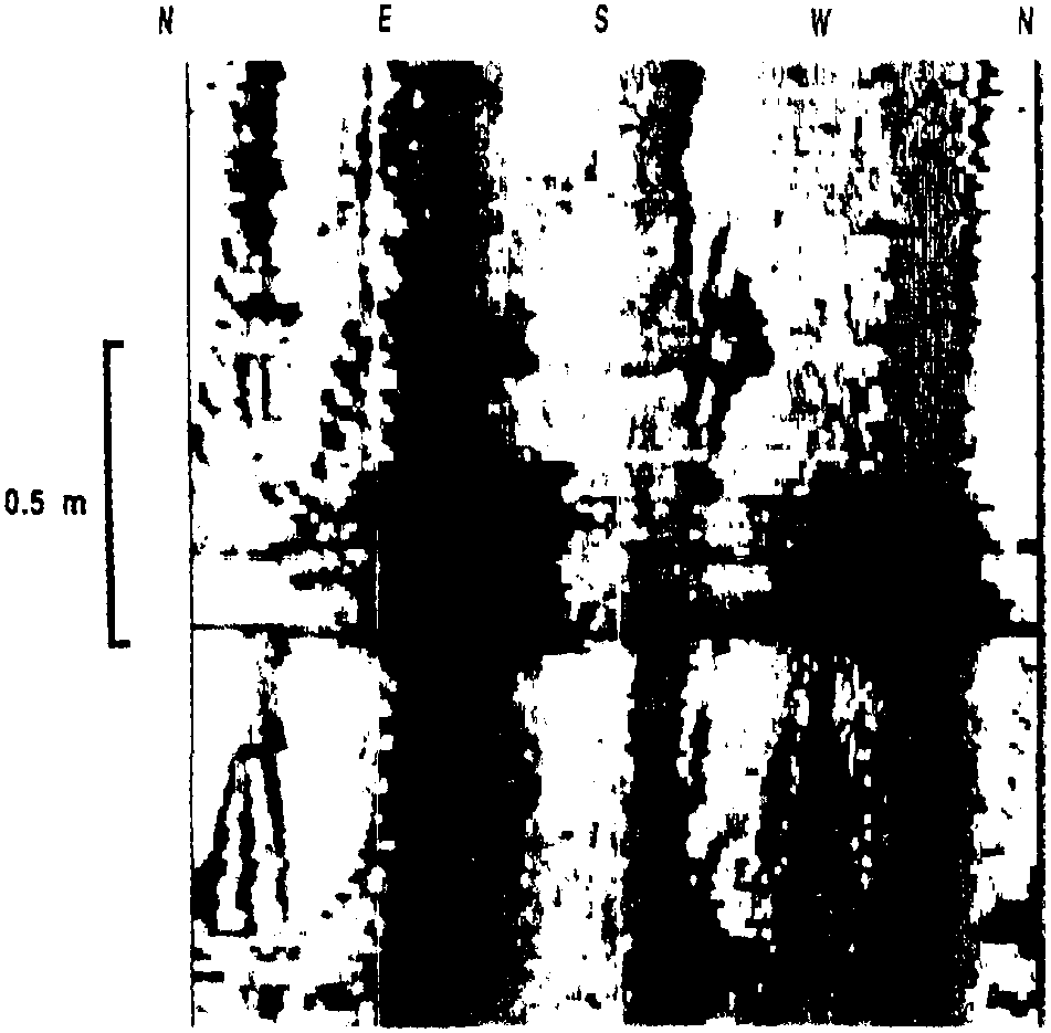
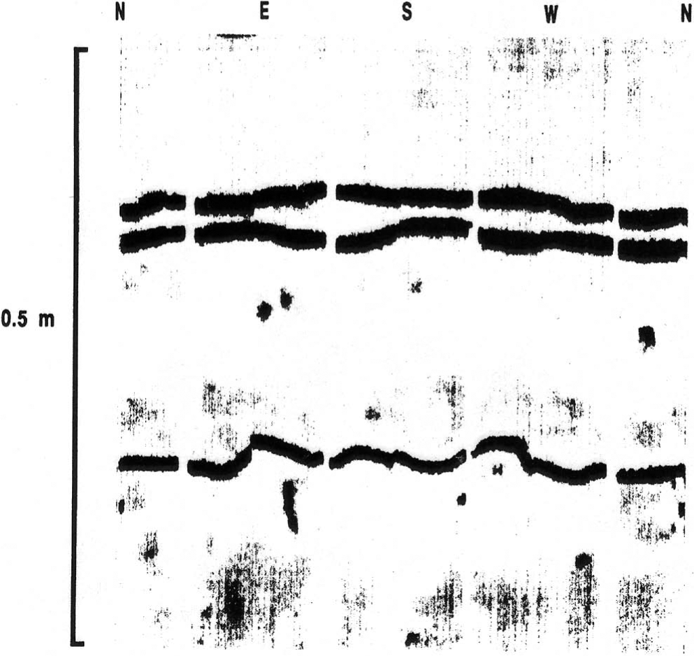
25 KB | Borehole televiewer image showing breakouts (dark patches) at NNW and SSE. Category:Wireline methods | 1 |
| 18:53, 13 January 2014 | Borehole-imaging-devices fig6.png (file) |  |
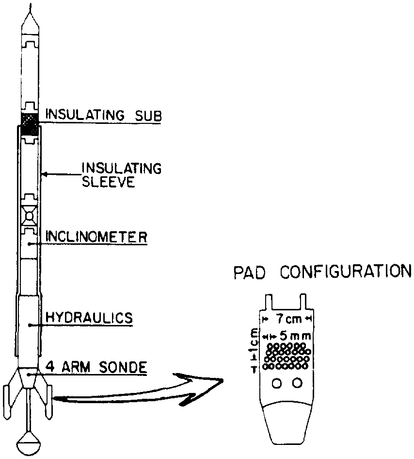
12 KB | Formation MicroScanner technique. (From Ekstrom et al., 1987.) Category:Wireline methods | 1 |
| 18:53, 13 January 2014 | Borehole-imaging-devices fig7.png (file) |  |
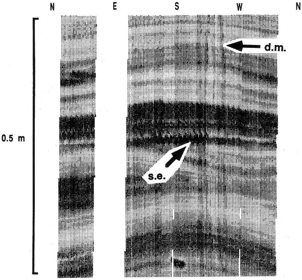
508 KB | Formation MicroScanner images of cross-bedded sequence showing drill marks (d.m.) at WSW and sawtooth effects (s.e.) on some layers. Category:Wireline methods | 1 |
| 18:53, 13 January 2014 | Borehole-imaging-devices fig8.png (file) |  |
416 KB | Formation MicroScanner images showing dipping unconformity at contact (arrow) of Cretaceous clastic rocks with Mississippian carbonates. Category:Wireline methods | 1 |
| 18:53, 13 January 2014 | Borehole-imaging-devices fig9.png (file) |  |
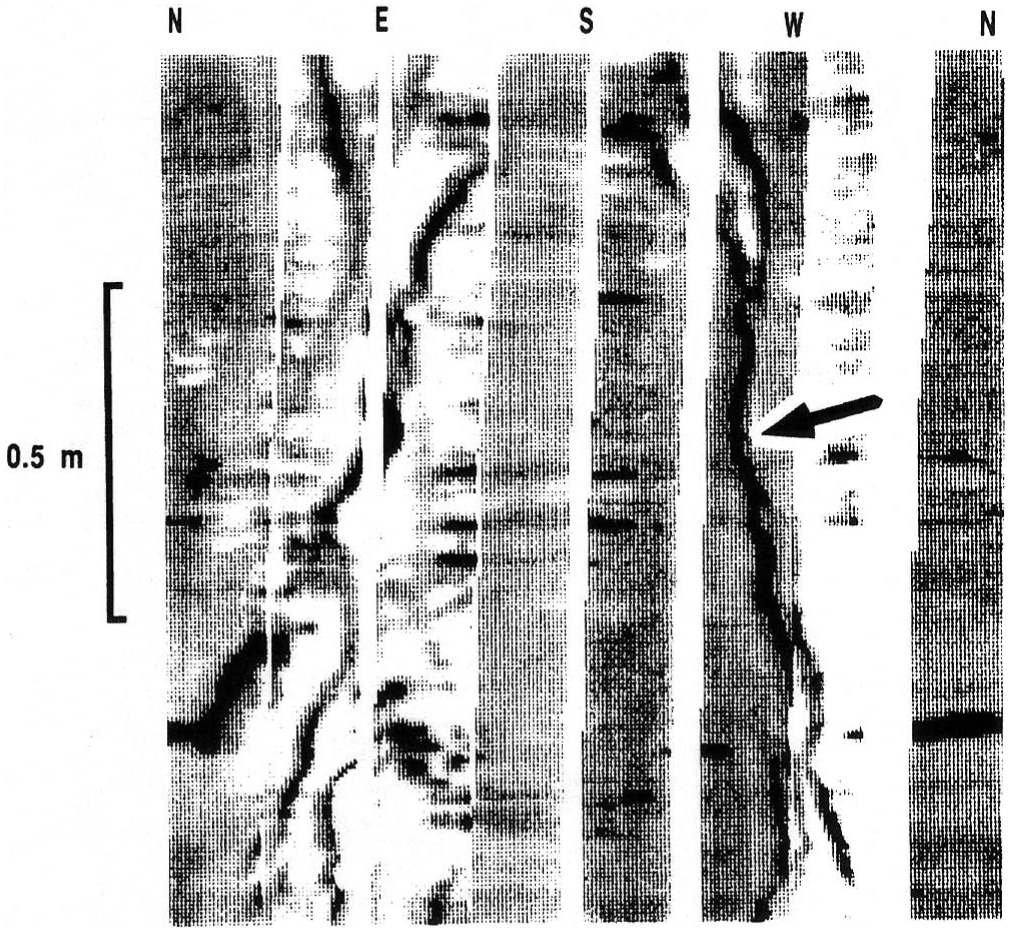
561 KB | Formation MicroScanner images of open conductive fracture (arrow). Category:Wireline methods | 1 |
| 18:53, 13 January 2014 | Borehole-imaging-devices fig10.png (file) |  |
271 KB | Formation MicroScanner images of stylolitic limestone. Category:Wireline methods | 1 |
| 19:02, 13 January 2014 | Carbonate-reservoir-models-facies-diagenesis-and-flow-characterization fig1.png (file) |  |
53 KB | Dunham (1962) classification of carbonate rocks according to depositional texture. (From Swanson, 1981.) Category:Geological methods | 1 |
| 19:02, 13 January 2014 | Carbonate-reservoir-models-facies-diagenesis-and-flow-characterization fig2.png (file) |  |
136 KB | Carbonate depositional environments. (Diagram by R. G. Loucks and C. R. Handford, unpublished.) Category:Geological methods | 1 |
| 19:02, 13 January 2014 | Carbonate-reservoir-models-facies-diagenesis-and-flow-characterization fig3.png (file) |  |
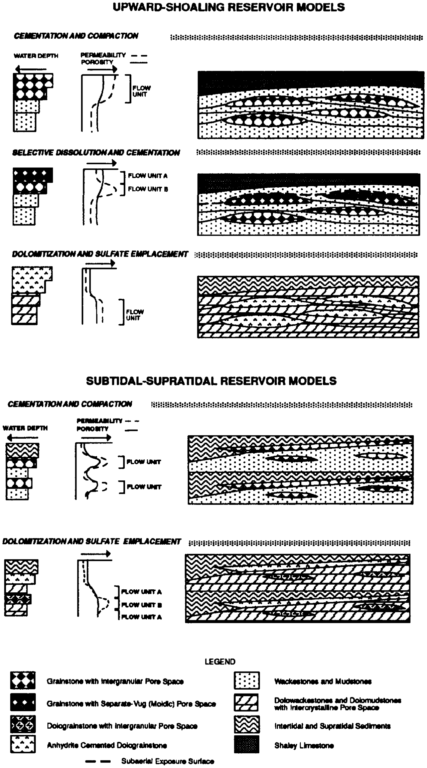
219 KB | Schematic diagrams of the upward-shoaling cementation and compaction reservoir model and the subtidat-supratidal dolomitlzation and sulfate emplacement reservoir model. Category:Geological methods | 1 |
| 19:02, 13 January 2014 | Carbonate-reservoir-models-facies-diagenesis-and-flow-characterization fig4.png (file) |  |
189 KB | Schematic diagram of the karst-collapse reservoir model showing three karst facies. (From Kerans, 1989.) Category:Geological methods | 1 |
| 21:28, 13 January 2014 | Checkshots-and-vertical-seismic-profiles fig1.png (file) |  |
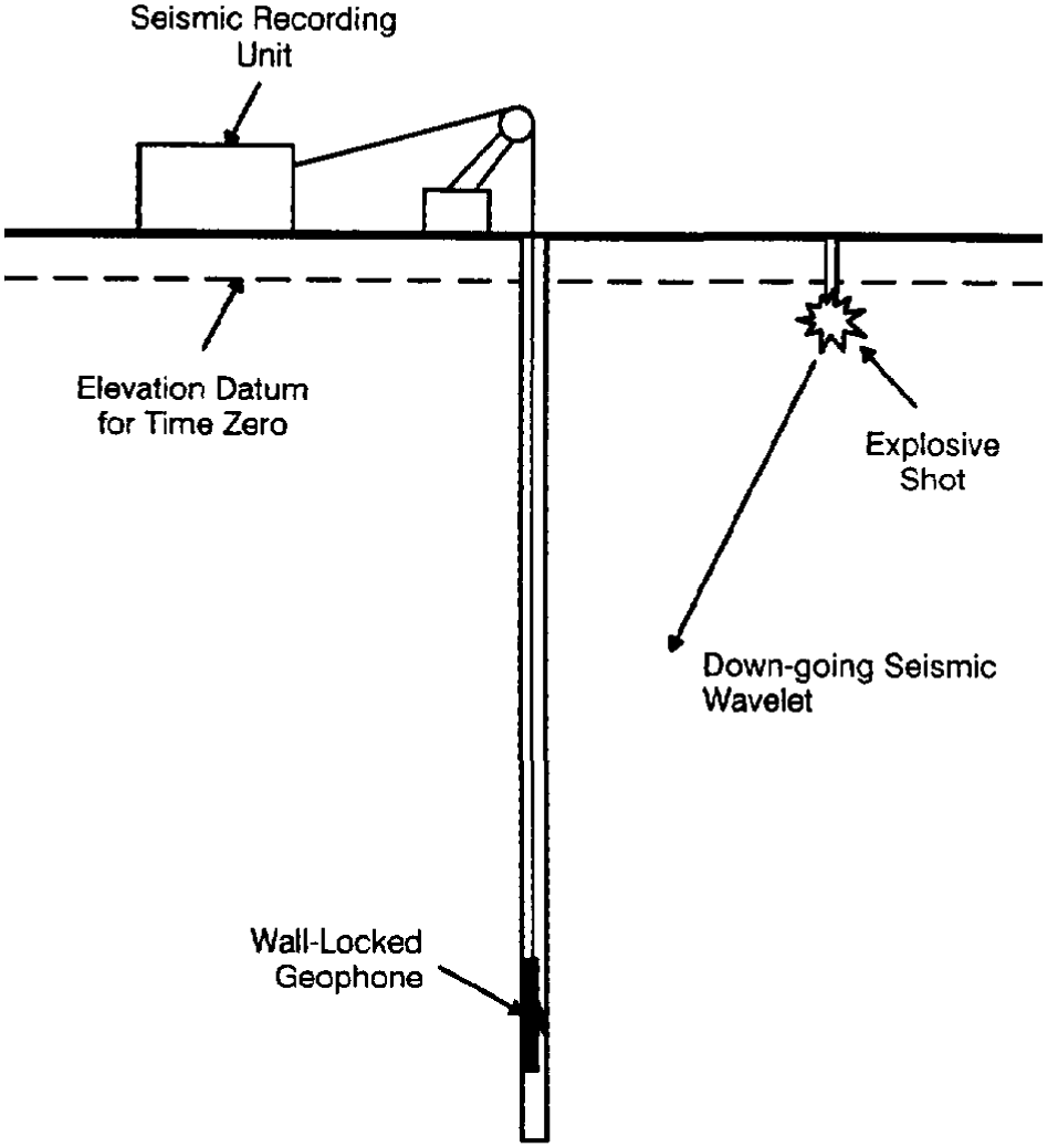
24 KB | The source-receiver geometry commonly used in onshore checkshot surveys. Category:Geophysical methods | 1 |
| 21:28, 13 January 2014 | Checkshots-and-vertical-seismic-profiles fig2.png (file) |  |
12 KB | The source-receiver geometry commonly used to record checkshots in deviated wells. Category:Geophysical methods | 1 |
| 21:28, 13 January 2014 | Checkshots-and-vertical-seismic-profiles fig3.png (file) |  |
8 KB | The source position (A or B) should be chosen so that the travel path to each receiver is as nearly vertical as possible. Category:Geophysical methods | 1 |
| 21:29, 13 January 2014 | Checkshots-and-vertical-seismic-profiles fig4.png (file) |  |
56 KB | Examples of the source-receiver positions involved in (a and b) zero offset and (c and d) offset VSP recording geometries. Category:Geophysical methods | 1 |
| 21:36, 13 January 2014 | Lithofacies-and-environmental-analysis-of-clastic-depositional-systems fig1.png (file) |  |
21 KB | Sedimentary processes, lithofacies, and lithofacies associations for a meandering channel sequence. (The vertical sequence is modified from Walker and Cant, 1984.) Category:Geological methods | 1 |
| 21:36, 13 January 2014 | Lithofacies-and-environmental-analysis-of-clastic-depositional-systems fig2.png (file) |  |
16 KB | Gamma ray correlation (dip section) of a series of prograding shoreface sandstones. Note the imbricate nature of the sandstone bodies and the “non-layer cake” nature of the correlations. Category:Geological methods | 1 |
| 21:37, 13 January 2014 | Lithofacies-and-environmental-analysis-of-clastic-depositional-systems fig3.png (file) |  |
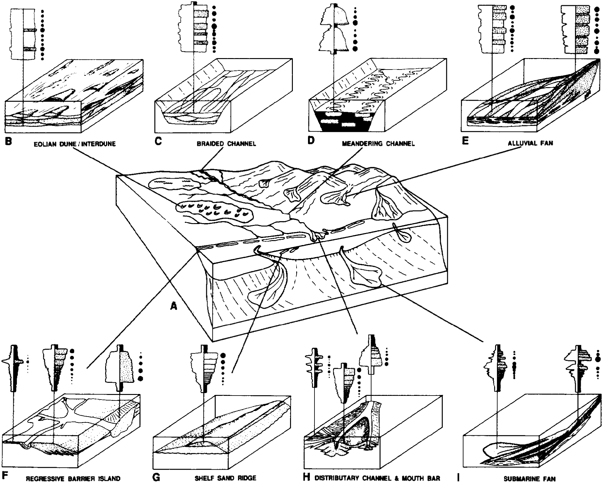
201 KB | Models of major depositional environments. The curve on the left shows the SP or gamma ray response and the curve on the right shows the relative grain size profile. The size of the dots next to the vertical profile indicates the relative magnitude of ... | 1 |
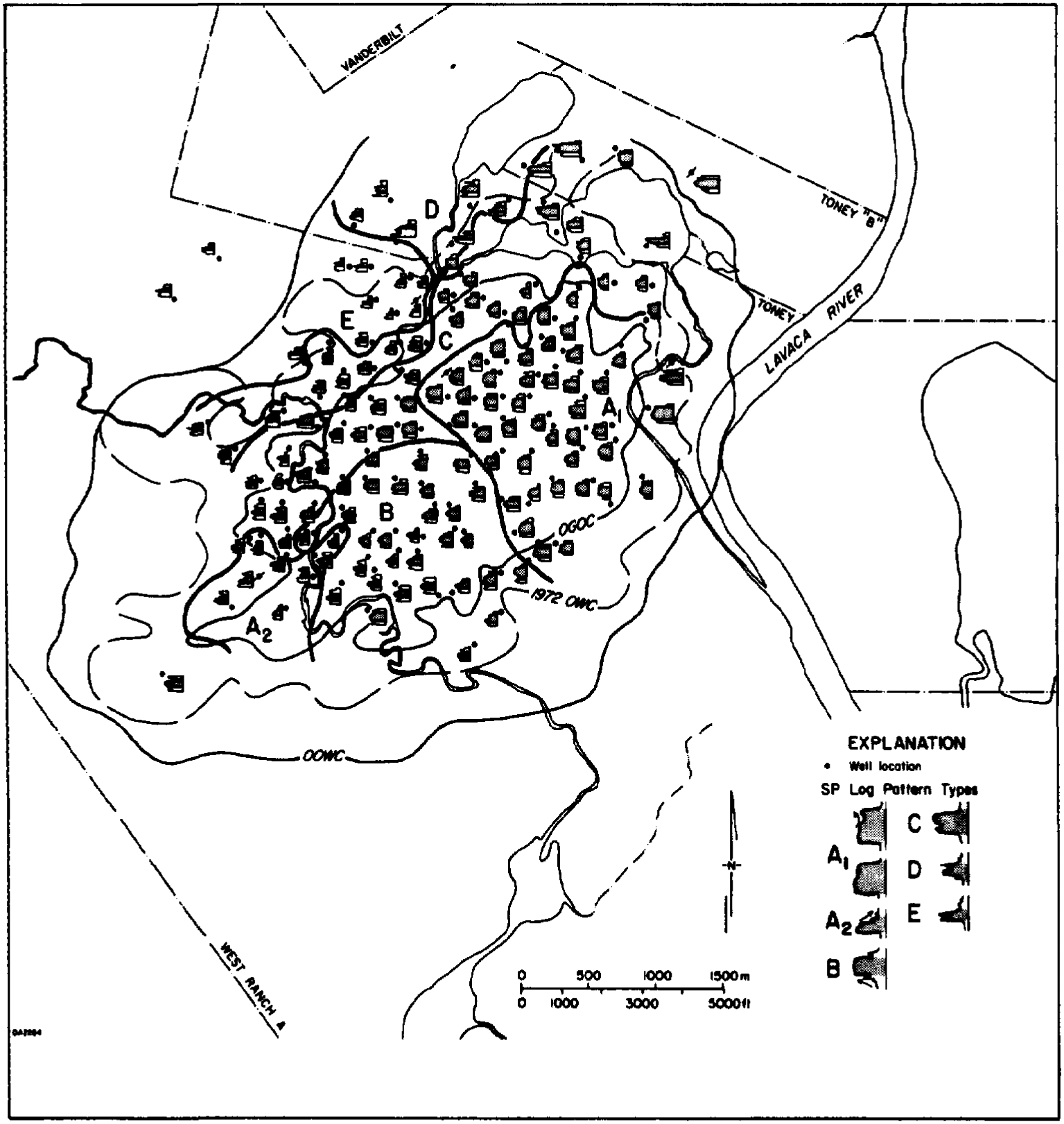
| 22:02, 13 January 2014 | Evaluating-stratigraphically-complex-fields fig1.png (file) |  |
139 KB | Example of electrofacies map showing distribution of SP log patterns. (From Galloway and Cheng, 1985.) Category:Geological methods | 1 |
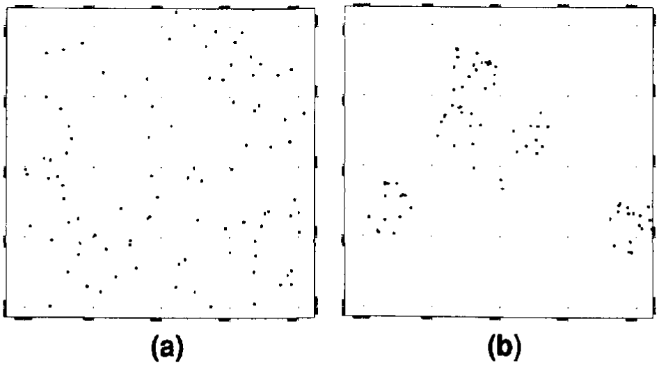
| 22:06, 13 January 2014 | Introduction-to-contouring-geological-data-with-a-computer fig1.png (file) |  |
13 KB | (a) Random points. (b) Clustered points. Category:Integrated computer methods | 1 |
| 22:06, 13 January 2014 | Introduction-to-contouring-geological-data-with-a-computer fig2.png (file) |  |
23 KB | Triangular mesh prepared from Davis (1973) data. Category:Integrated computer methods | 1 |
| 22:06, 13 January 2014 | Introduction-to-contouring-geological-data-with-a-computer fig3.png (file) |  |
21 KB | Contoured triangular mesh of Figure 2. Category:Integrated computer methods | 1 |
| 22:06, 13 January 2014 | Introduction-to-contouring-geological-data-with-a-computer fig4.png (file) |  |
53 KB | Surface contoured on a triangular mesh. The original surface is a fourth-order polynomial. Category:Integrated computer methods | 1 |
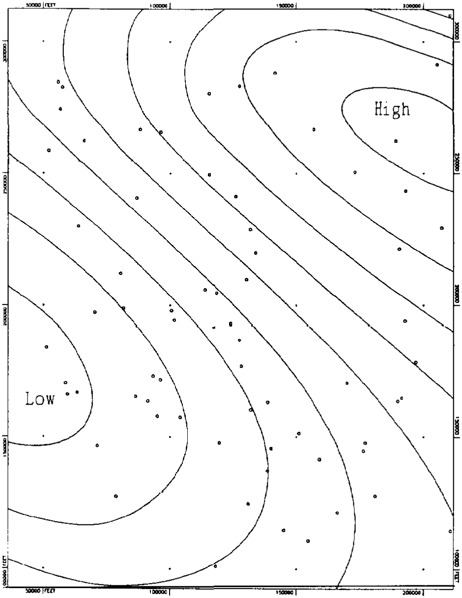
| 22:06, 13 January 2014 | Introduction-to-contouring-geological-data-with-a-computer fig5.png (file) |  |
63 KB | Contours from a 13 × 13 grid using nearest neighbor search. (Data from Davis, 1973.) Category:Integrated computer methods | 1 |
| 22:06, 13 January 2014 | Introduction-to-contouring-geological-data-with-a-computer fig7.png (file) |  |
51 KB | A representation of the fourth-order polynomial of Figure 4 contoured on a grid prepared using a nearest neighbor search criterion. Category:Integrated computer methods | 1 |
| 22:06, 13 January 2014 | Introduction-to-contouring-geological-data-with-a-computer fig6.png (file) |  |
42 KB | A13 × 13 grid showing the relationship between grid nodes and control points for the Davis (1973) data set. Category:Integrated computer methods | 1 |
| 22:32, 13 January 2014 | Using-and-improving-surface-models-built-by-computer fig1.png (file) |  |
31 KB | Contour maps of the same surface data. (a) Unconstrained extrapolation into nondata areas. (b) Contours constrained to areas near data. Category:Integrated computer methods | 1 |
| 22:32, 13 January 2014 | Using-and-improving-surface-models-built-by-computer fig2.png (file) |  |
18 KB | Cross section showing the output from filtering being constrained between models built by shifting the initial surface model up and down slightly. Category:Integrated computer methods | 1 |
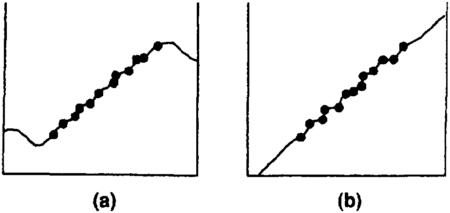
| 22:32, 13 January 2014 | Using-and-improving-surface-models-built-by-computer fig3.png (file) |  |
5 KB | Cross sections through the same data. (a) Extrapolated values for a weighted average algorithm tend to “come back” to the average of near data values. (b) Acceptable surface extrapolation achieved by creating a first-order trend, modeling residuals... | 1 |
| 22:32, 13 January 2014 | Using-and-improving-surface-models-built-by-computer fig4.png (file) |  |
5 KB | Cross sections through the same data. (a) The surface model does not honor the data. (b) Surface is shifted to data by modeling the error between the data and the original surface and then adding the original and error models. [[Category:Integrated co... | 1 |
| 22:32, 13 January 2014 | Using-and-improving-surface-models-built-by-computer fig5.png (file) |  |
11 KB | Contour maps of the same data. (a) Most algorithms weight data isotropically and creat circular surface forms. (b) Single direction bias forces elliptical weighting, allowing surface form to stretch in one direction. [[Category:Integrated computer met... | 1 |
| 22:32, 13 January 2014 | Using-and-improving-surface-models-built-by-computer fig6.png (file) |  |
12 KB | Cross section showing two conformable surfaces. Dashed line represents direct modeling of lower surface data. Solid lines represent direct modeling of upper surface data and conformable modeling of lower surface data. [[Category:Integrated computer me... | 1 |
| 22:32, 13 January 2014 | Using-and-improving-surface-models-built-by-computer fig7.png (file) |  |
12 KB | Cross section showing four conformable surfaces. The second from the top is the control and is modeled using structure data. The other surfaces are built using the conformable method. Category:Integrated computer methods | 1 |
| 22:32, 13 January 2014 | Using-and-improving-surface-models-built-by-computer fig8.png (file) |  |
9 KB | Cross sections showing that surfaces that intersect due to (a) baselap or (b) truncation will incorrectly cross one another. Category:Integrated computer methods | 1 |
| 22:32, 13 January 2014 | Using-and-improving-surface-models-built-by-computer fig9.png (file) |  |
5 KB | Cross sections showing a baselapping surface (a) as coincident with the lower surface in areas of baselap (for cross section display) and (b) as missing in areas of baselap (for map display). Category:Integrated computer methods | 1 |
| 22:32, 13 January 2014 | Using-and-improving-surface-models-built-by-computer fig10.png (file) |  |
5 KB | Cross section showing surfaces before baselap operations. The zero contour of the model built by subtracting the two surfaces defines the subcrop line. Category:Integrated computer methods | 1 |
| 22:32, 13 January 2014 | Using-and-improving-surface-models-built-by-computer fig11.png (file) |  |
13 KB | Map showing contours and subcrop lines. Category:Integrated computer methods | 1 |