Drill stem testing

Development Geology Reference Manual
Series	Methods in Exploration
Part	Wellsite methods
Chapter	Drill stem testing
Author	Ingrid Borah
Link	Web page
Store	AAPG Store

A drill stem test (DST) is a temporary completion of a wellbore that provides information on whether or not to complete the well. The zone in question is sealed off from the rest of the wellbore by packers, and the formations' pressure and fluids are measured. Data obtained from a DST include the following:

• fluid samples
• reservoir pressure (P*)
• formation properties, including permeability (k), skin (S), and radius of investigation (r_i)
• productivity estimates, including flow rate (Q)
• hydrodynamic information

This article focuses on nonflowing DSTs (NFDSTs). In a NFDST, fluid does not flow to the surface and a stabilized flow rate is not obtained (also, the well can flow to the surface but die or be shut-in before steady-state rates are achieved). Analysis of flowing DSTs is less complicated because flow rates can be measured throughout the test.

Planning

Figure 1 Drill stem test tool string.

The key to successful testing depends upon planning and teamwork between the geoscientist and the engineer. Potential pay zones should be identified before drilling commences so that the drilling program can be designed to accommodate the test. If offset data are available, the magnitude of porosity, permeability, and reservoir pressure should be identified. Knowledge of zonal mineralogy may prevent excessive damage by drilling fluids and should be used in designing the mud program. The anticipated reservoir properties are used to design the test string and test times so that the best, most useable data can be obtained.

Safety

Running a DST is one of the most dangerous jobs in the oil field because the well is essentially uncontrolled during the test. All fire fighting equipment and the blowout preventers should be inspected and tested before starting a DST. Hydrogen sulfide (H₂S) equipment should be on hand if anticipated conditions are sour. No test should be initiated at night or during an electrical storm. No smoking should be allowed on the drill floor or near any flowlines or surface test equipment.

Packer seats

The best time to run a DST is just after drilling through a potential pay zone, when exposure to damaging fluids is minimal and the hole is in its best condition for a good packer seat. Packer seats are generally located in competent sandstones or carbonates above the test interval or both above and below it. The packer seat is picked by the geoscientist or mudlogger using cuttings and the rate of penetration (ROP) as guides. Soft formations, characterized by a fast ROP, usually do not make good packer seats because the packer has trouble seating or gripping the side of the borehole. This results in poor pressure seals, or in extreme cases, the packer may slide down the hole.

Length of test interval

The length of the test interval should be short so that less mud will be displaced from the rathole (the portion of the open hole below the bottom packer) into the drill string.

Length of test time

The length of flow and shut-in periods during the test are critical to obtaining good reservoir data. The dual flow, dual shut-in test is most commonly used. The initial flow period of 3-5 min removes the “supercharge” effect of mud filtrate near wellbore. The first buildup is run for 60 min to determine a valid P* (reservoir pressure). The second flow period is used to collect a fluid sample and create a pressure disturbance at a distance beyond any damaged zone. The duration of the final flow period may be anywhere between 60 and 120 min, depending upon the time available for the test and the final buildup. The final buildup is used to evaluate reservoir transmissibility, damage, and radius of investigation and should be at least as long as the final flow period. It is preferable (daylight permitting) to run the final build up three times as long as the final flow period to ensure that good pressure transient data is recorded.

Mud system

If a drill stem test is anticipated, low fluid loss mud will prevent excessive leakoff into the target zone and doping the mud with nitrates will distinguish filtrate from recovered formation water.

Test tools

A drill stem test string consists of packers, a downhole shut-in valve, a safety joint, and pressure gauges (Figure 1). The bottom packer and blanked off gauge are shown as an “add on” to a straddle test.

Figure 2 Straddle drill stem test tool string. (a) Typical MFE inflate open hole string (straddle, off-bottom). (b) Typical MFE straddle string (open hole, conventional, off-bottom). (From Flopetrol-Johnston.)

Packers

Compression set packers are generally more reliable than inflatable packers because they can withstand more differential pressure between the annulus and the drill string. The number of packers depend upon experience and test type (conventional, straddle, or hookwall. Figure 2 illustrates other types of test strings.

Packer selection is also determined by the need for a cushion. A cushion consists of water or gas and is run for the following reasons:

• To prevent drill string collapse during deep tests or when high mud weights are used
• To prevent excessive differential pressure across the packer(s) during the flow periods
• To prevent high differential pressure across the sand face in unconsolidated formations, which will result in sand flow
• To prevent corrosion of the drill string from corrosive gases such as H₂S or CO₂

Cushions also provide back pressure on the formation, which inhibits flow into the test string. If considerable damage or low permeability is expected, the cushion should be small.

Pressure gauges

A minimum of three (mechanical, electronic, or a combination) pressure and temperature recorders should be run on a conventional test and four on a straddle test. Selection depends on how accurate the data need to be.

One gauge should always be run inside the drill string above the closing tool. This gauge measures the hydrostatic head of fluid produced into the drill pipe and is critical to evaluating the volumes of fluids produced during the test. It also indicates drill string leakage during the test.

Two gauges should be run below the closing tool to measure pressure during the flow and shut-in periods. Two are needed to verify that they are reading within their calibration ranges and to provide a backup in case one fails.

A blanked off gauge must be run on a straddle test to verify that the bottom packers were holding. In most cases of straddle test failure, it is the bottom packers that fail.

Analyzing the DST

• 

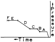
  Figure 3 Perfect chart. Gauge located inside and above the closing tool. (A) Add cushion/run in hole; (B) initial flow period; (C) initial shut-in period; (D) final flow period; (E) final shut-in period; and (F) pulling out of hole.

• 

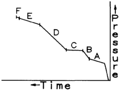
  Figure 4 Collar leak. Gauge located inside and above the closing tool. Chart indicates increasing pressure during running in hole and shut-in periods.

• 

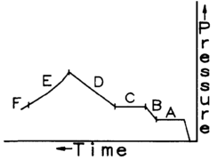
  Figure 5 Fluid loss from drill pipe. Gauge located inside and above the closing tool. Bleeder valve on drill string left open during shut-in periods.

• 

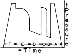
  Figure 6 Perfect chart. Gauges inside above and outside below the closing tool. Pressure transient analysis done from these gauges. (A) Run in hole, gauge measuring hydrostatic pressure of mud column; (B) initial flow period; (C) initial buildup; (D) final flow period; (E) final buildup; and (F) release packer and pulling out of hole.

• 

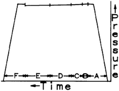
  Figure 7 Perfect chart. Blanked off gauge below the bottom packer on a straddle test. (A) running in hole; (B) initial flow period; (C) initial buildup; (D) final flow period; (E) final buildup; and (F) pulling out of hole.

• 

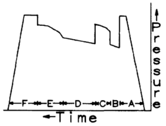
  Figure 8 Bottom packer failure. Blanked off gauge below bottom packer on a straddle test. When the bottom packer fails, the pressure gauge will read some flow and buildup data but will not replicate gauges run above the bottom packer because of a restricted flow area around the packer elements. (Types of gauge failures are described in .)

Once the drill stem test is concluded, mechanical validity and fluid recovery must be verified.

DST chart analysis

Descriptions of valid DST charts are shown in Figures 3, 4, 5, 6, 7, and 8. (See figure captions for discussion.)

Fluid recovery (Nonflowing Test)

On an NFDST, the volume of fluid produced from the formation is contained in the drill string. A fluid level must be determined to calculate the volume recovered. If the fluid is highly gas-cut, a straight volume calculation will be inaccurate. Therefore, samples should be collected at regular intervals while reversing to a clean tank on location. Although it is common to reverse to a pit, the amount of fluid recovered cannot be determined if this is done. Error in measuring fluid recovery often makes the difference between an economic disaster or a success. Also, grindouts (centrifuge) must be performed on each sample to determine the percentage of oil, water, and solids. Resistivity, chloride content, and nitrate content of produced water and the specific gravity of all phases should be measured.

Estimating flow rates (Nonflowing Test)

During the flow period on a DST, the flow rate is not constant. A flow rate can be calculated using pressure data from the gauge above the shut-in tool. By dividing the time scale into discrete increments and recording the pressure, the data can be transposed to a position in the drill pipe. Since the volume of the drill string and the changing fluid composition are known, instantaneous flow rates can be calculated as shown in Table 1.

Table 1 Calculation of instaneous flow rates

dP/dT (psi/min)	Fluid Gradienta (psi/ft)	Flow Rate (BPD)
( P1 – P0 )/( t1 – t0 )	G1	(Col 1 ÷ Col 2) × 1440 × DPV
( P2 – P1 )/( t2 – t1 )	G2	(Col 1 ÷ COI 2) × 1440 × DPV
( Pn – Pn –1 )( tn – tn –1 )	Gn	(Col 1 ÷ Col 2) × 1440 × DPV

Other methods include the following:

• Superposition uses the rate schedule in analyzing the pressure data. The technique is described in Earlougher and in Matthews and Russell.
• The Odeh-Selig method (modified superposition) is fairly rigorous. It is only valid if the shut-in period is 1.5 times greater than the flowing period.
• The modified Horner method uses effective flow time and a flow rate calculated from the end of the second flow period. The effective flow time is calculated by dividing the total fluid recovery in barrels by the flow rate in barrels per minute, which is then converted to barrels per day.
• The simplified Horner method converts total recovery and the flow time of the test to an average daily rate. The flow time using this method is the time the tool was open. Although this method is commonly used, it is incorrect to assume that this rate reflects stabilized producing rates. This method should only be used as a last resort.

Interpretation

The most important parameters in DST interpretation are the radius of investigation (ROI) and the observed wellbore storage constant (WBSC). A short ROI, combined with knowledge of drilling fluid properties (fluid loss or amount of overbalance), may indicate that the calculated permeability is indicative of only the damaged zone. Usually, a skin factor close to zero is calculated under these conditions, along with a low formation transmissibility (kh/μ). One way to “see” past this damaged zone is to rerun the drill stem test with longer flow and shut-in periods.

If fractures are present, the measured WBSC may be much higher than the calculated WBSC. A high transmissibility and a negative skin will be computed under these conditions. A negative skin implies stimulation, which cannot occur during normal drilling operations. If an interval is fractured, recoveries and calculated flow rates can be much greater than expected future production.

Calculating wellbore storage capacity

To calculate the wellbore storage capacity (WBSC), plot log (P_ws – P_wf) versus log (t_s – t_wf) (terms defined in Table 2). Because of storage effects, the early portion of the data will have a unit slope. As these effects diminish, data points on the log-log plot fall below the unit slope line and approach the slowly curving line for no wellbore storage. The measured WBSC (WBSC_meas) is calculated using one point from the unit slope line in the following equation:

${\mbox{WBSC}}_{\rm {meas}}={\frac {Q_{\rm {last}}B_{\rm {o}}\Delta t}{1440\Delta P}}$

(See Table 2 for explanation of mathematical variables.)

Table 2 Nomenclature of mathematical variables

Variable Symbol	Explanation	Units
Pw s	Pressure during the shut-in	psi
Pwf	Final flowing pressure	psia
t0	Time during shut-in	minutes
twf	Time at last flowing pressure	minutes
ts	Shut in time	minutes
Qlast	Last flow rate	stb/day
Δ t	Time difference	minutes
Δ P	Pressure difference	psi
Vrh	Volume of the rathole below the packer	bbl
h	Sand thickness	ft
μ	Fluid viscosity	cp
q	Producing rate	stb/day
P *	Reservoir pressure determined from buildup #1	psia
Pave	Average flowing pressure	psia
m	Slope from Horner plot	psi/cycle
k	Permeability	md
t	Flow time (in skin equation)	hr
φ	Porosity	decimal
Ct	System compressibility	psi–1
rw	Wellbore radius	ft
kh lμ	Transmissibility	md-ft/cp
re	Estimated drainage radius	ft
Bo	Formation volume factor	bbl/stb
S	Skin term	(dimensionless)
WBSCcalc	Calculated wellbore storage constant	bbl/psi
WBSCmeas	Measured wellbore storage constant	bbl/psi
G1 , G2 , Gn	Gradients of individual fluid samples	psi/ft
P0 ,. P1 , P2 , Pn	Flowing pressures at times t0 , t1 t2 , tn	psi
t0 , t1 , t2 , tn	Flowing times	minutes

The calculated WBSC (WBSC_calc) is computed as follows:

${\mbox{WBSC}}_{\rm {calc}}={\frac {V_{\rm {rh}}}{P_{\rm {wf}}}}$

Calculating static reservoir pressure

Figure 9 Horner plot.

Reservoir pressure (P*) is calculated by extrapolating the pressure data (from the first buildup on a DST) on the Horner (or superposition) plot to an infinite shut-in rime (Figure 9). This pressure provides a guide for selecting the slope of the second buildup Horner plot. If the second buildup slope extrapolates to a pressure significantly less than P*, depletion might be suspected. To see true depletion, the reservoir would have to be very small. Although depletion is possible in rare cases, identifying it is usually a result of poor test design and analysis.

A method for constructing the Horner plot is outlined as follows. After determining the effective producing time and producing rate, tabulate time and pressure for each buildup period. Make plots using Cartesian paper because this makes it easier to expand the plot (see Figure 9). Now plot P versus log[(t + Δt)/Δt] for buildup #1 (the first buildup following the first flow period). Note that t in this equation is equal to the length of the initial flow period and that Δt is the time since the start of the buildup period.

Extrapolate this curve to P* at log[(t + Δt)/Δt] = 0. P* provides the “guiding light” for determining the proper slope found using buildup #2. Now plot P versus log[(t + Δt)/Δt] for buildup #2. Note here that this t is the effective producing time calculated from one of the methods outlined earlier.

Extrapolate the straight-line portion of the data to P*. Use a data band within the accuracy of the gauge to make sure you choose the correct slope. In other words, if the gauge is accurate within ±5 psig, then the data band should be 10 psi wide on the graph. A data band is extremely important in cases where m m using two points: (x₁, y₁) and (x₂, y₂), where

$m={\frac {y_{2}-y_{1}}{x_{2}-x_{1}}}$

Now calculate the formation transmissibility as follows:

${\frac {kh}{\mu }}={\frac {162.6qB_{\rm {o}}}{m}}$

Note that k/μ can be calculated directly from the transmissibility term if the thickness, h, is known. Also, if a good value for μ is known, the formation capacity, kh, can be determined.

Calculating skin factor

The skin factor (S) can be calculated as follows:

$S=1.151\left[{\frac {{\big (}P^{*}-P_{\rm {ave}}{\big )}}{m}}-\log \left({\frac {kt}{\phi \mu c_{\rm {t}}r_{\rm {w}}^{2}}}\right)+3.23\right]$

If fluid properties are unavailable, skin can be calculated assuming that the log term in the previous equation is equal to 7.5. In most cases, the skin will either be positive or close to zero. A negative skin greater than –1 should be viewed with caution since the well has not been stimulated.

Calculating radius of investigation

The radius of investigation (ROD is important because it helps determine whether or not the test saw beyond wellbore damage. It is defined as

$r_{\rm {i}}={\frac {1}{2}}{\sqrt {\frac {1.05\times 10^{-3}kt}{\phi \mu c_{\rm {t}}}}}$

where t is the buildup time in hours and all other terms have been previously defined. The ROI calculated from a DST should not be used to identify faults or boundaries. If such items are in question, they should be determined through further transient testing.

Using the pseudo-steady-state radial flow equation, the potential of the tested interval can be estimated as follows:

$q=0.00708\left({\frac {kh}{\mu }}\right)\left[{\frac {{\big (}P^{*}-P_{\rm {wf}}{\big )}}{B_{\rm {o}}\left(\ln \displaystyle {\frac {r_{\rm {e}}}{r_{\rm {w}}}}-\displaystyle {\frac {1}{2}}+S\right)}}\right]$

Note that P_wf in this case is the assumed drawdown by pumping or flowing. It is not the same flowing pressure seen on the DST. Also, the skin factor S here may be the skin expected after cleanup or stimulation.

Common pitfalls in Dst testing and analysis

All too often, DSTs are run for fluid recovery instead of for reservoir data. Flowing test times are long and shut-in times short. Producing rates are calculated using the simplified Horner method and can be overly optimistic. Even in DSTs in which the test times are run as recommended, incorrect estimation of fluid recovery can lead to incorrectly calculated flow rates used in reservoir calculations. Care should be taken to analyze the test. For example, a recovery of length::50 ft of oil-cut mud might indicate that a zone was too damaged to produce and not that it was tight!

Examples of practical Dst analysis

Example 1: Calculation of flow rates

Well	Number 26-1
Location	Roosevelt County, Utah
Test Interval	5910–6011 ft
	Green River Formation
Test Results	Highly gas-cut oil flowed to surface. Stabilized rate was not obtained. Estimated recovery (drill string volume reversed to pit) was 54 bbl of oil and 5 bbl of mud. Test was analyzed using the three methods outlined in Table 3, which shows calculated reservoir parameters.

As can be seen in Table 3, flow rates vary widely depending upon the method used. The calculated steady-state producing rate was 181 BOPD using the superposition method. The actual producing rate for this well was 120 BOPD. The negative skin indicates a fracture system. The ROI was far enough away from the wellbore to see true reservoir permeability. Despite the excellent DST recovery, this well had projected reserves of 50,000 bbl of oil, which did not pay for drilling and completion costs.

Table 3 Example 1: impact of flow rates on reserve parameters

Method	Calculated Flow rate (bbl/day)	Producing Time (hrs)	Permeability (md)	Skin	ROI (ft)	Reservoir Pressure (psia)
Superposition	1313 → 192	1	6.6	–4.5	37	2405
Odeh–Selig	454	2.9	9.6	–3.6	—	—
Simplified Horner	1426	1	13.1	–4.1	53	2405

Example 2: Incorrect estimation of recovery without verifying recovery

Well	Number 17-1
Location	Williston Basin
Test Interval	8549–8639 ft
	Duperow
Test Results	Pipe was pulled to the fluid in the drill pipe. The DST report indicated a recovery of depth::1575 ft of highly oil and gas-cut water at a 60% oil-cut (11.5 bbl oil and 7.7 bbl water according to pipe measurements). Total flow time on the test was 1 hour. The well was completed, fractured, and plugged after testing less than 30 BFPD. This well should have been plugged after the DST. Pressure data from the gauge above the closing tool indicated that during the flow periods, the fluid pressure in the drill string increased by 115 psig. An oil gravity of 42° API was recorded from the sample chamber. A gradient of 0.389 psi/ft was calculated for the fluid mixture in the drill pipe. A fluid column of length::295 ft of un-gas-cut fluid was recovered in the drill string. This translated into an actual recovery of 1.8 bbl of fluid (1.08 bbl oil and 0.72 bbl water).

The fact that the drilling fluid was highly gas-cut led to an erroneous estimate of fluid recovery and unnecessary investment. It is always important to verify recovery using gauge data and field measured fluid densities.

Example 3: Basing potential productivity on recovery

Wells	34 and 65
Location	Sussex Field
	Johnson County, Wyoming
Test Results	These two wells were drilled in the early 1950s and tested the Shannon sand at approximately depth::4600 ft. The test tools were open for about 1 hour and shut-in for 30 minutes. In both cases, less than length::50 ft of oil-cut mud was recovered. Both wells were plugged on the basis of recovery.

Several years later, four offsets were drilled and had initial potentials greater than 200 BOPD after being hydraulically fractured in the same zone. In wells 34 and 65, the formation had been too damaged to produce during the DST. Both wells would have been productive after stimulation had the pressure data been analyzed on these tests.

See also

• Show evaluation
• Pressure detection
• Introduction to wellsite methods

External links

find literature about Drill stem testing

• Original content in Datapages
• Find the book in the AAPG Store

drill stem test

return on investment

barrels