Seismic data - creating an integrated structure map

Exploring for Oil and Gas Traps
Series	Treatise in Petroleum Geology
Part	Predicting the occurrence of oil and gas traps
Chapter	Interpreting seismic data
Author	Christopher L. Liner
Link	Web page
Store	AAPG Store

Below is a recipe for making a classic integrated structure map from seismic data and well control. It is based on mapping one horizon at a time and must be repeated for each horizon of interest. It may not work in areas with severe static problems (i.e., lots of topography or a rapidly changing weathered layer such as glacial till). It also fails when there are extreme lateral velocity variations in the subsurface (subsalt, subthrust, etc.). When it works, this method gives a map which, by definition, matches every well exactly. It uses seismic time structure to interpolate between wells and extrapolate beyond them.

Procedure

Follow the steps listed below for each seismic event to be mapped.

1. Make structure contour maps for key horizons using well control only.
2. Pick seismic horizons.
3. Calculate depth conversion velocity at locations where both well and seismic time picks exist.
4. Convert time to depth by multiplying the time structure map and the depth conversion velocity map.
5. Contour the integrated structure map, keeping in mind the structure map made earlier from well data only.

Step 1: Map structure from well data

Post well depths to key horizons and contour structure maps for key horizons using well control only. These well maps of structure should guide you when making structure maps that integrate both well and seismic data. Comparing this map with the final time structure map gives a good feel for the additional information supplied by the 3-D seismic section.

Step 2: Pick seismic horizons

• 

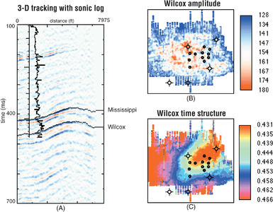
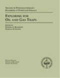
  Figure 1 (a) Representative line from the Glenn Pool data volume with sonic overlay and tracked events; (b) Horizon amplitude and time structure maps for the Wilcox. From Liner. Courtesy PennWell.

• 

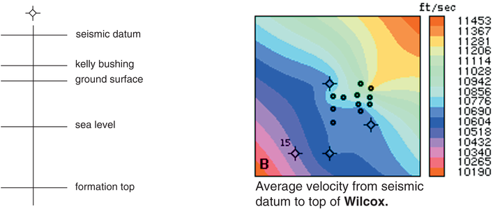
  Figure 2 Hypothetical well with important reference points; average velocity map for the Wilcox Formation in the Glenn Pool survey. From Liner. Courtesy PennWell.

• 

  Figure 3 Process and result for the Glenn Pool Wilcox horizon. From Liner. Courtesy PennWell.

For 2-D data, only the traveltime to each event of interest is recorded with its coordinate along the line t(x). For 3-D data, both traveltime and amplitude at each (x, y) are available from the seismic data cube, t(x, y) and a(x, y). The traveltimes form a time structure map, and the amplitudes are a horizon slice. Figure 1A shows a representative line from the Glenn Pool data volume with sonic overlay and tracked events. Horizon amplitude and time structure maps for the Wilcox are shown in Figures 1B, C.

Step 3: Calculate depth conversion velocity

Calculate depth conversion velocity at locations where both well and seismic time picks exist. The wells used as control do not need velocity or density logs but must penetrate the event of interest. The event depth z (measured from seismic datum) is known from well control, and the vertical reflection time t is known from the previous item. The depth conversion velocity is given by

$\upsilon ={\frac {2z}{t}}$

Depth conversion velocities are posted to a map and contoured or gridded to create υ(x, y).

Figure 2 shows a hypothetical well with important reference points as well the average velocity map for the Wilcox Formation in the Glenn Pool survey. This map has a fairly strong lateral velocity gradient, i.e., the velocity changes from about 11,400 ft/s for velocity (NE) to 10,200 ft/s (SW) in the space of just over a mile. When this occurs, time structure and depth structure can be significantly different.

Step 4: Convert time to depth

Convert time to depth by multiplying the time structure map and the depth conversion velocity map, i.e.,

$z(x,y)={\frac {\upsilon (x,y)\times t(x,y)}{2}}$

The factor of one-half is necessary because the times are two-way vertical times and we only want the one-way depth. Figure 3 shows the process and result for the Glenn Pool Wilcox horizon.

Step 5: Contour map

Figure 4 zoom of the central area in the maps in Figure 5. From Liner. Courtesy PennWell.

Contour or grid the integrated structure map with the same technique used for the wells-only depth map. This allows head-to-head comparison (Figure 4).

Integrated map

Figure 5 Comparison of the first depth map from well control only and the seismic plus well integrated depth map. From Liner. Courtesy PennWell.

The final product z(x, y) is called an integrated structure map. It honors all well-control depth points (by definition) and uses the seismic events to interpolate between these points. Figure 5 is a comparison of the first depth map from well control only and the seismic plus well integrated depth map.

Figure 4 is a zoom of the central area in the maps in Figure 5. Map A uses well control only, and map B uses well control plus seismic interpretation.

Conclusion

The mapping process described here can give useful results in many situations. However, the following cares should be considered:

• Strong lateral velocity variations may require depth migration and direct output to a depth cube.
• Existence of dense, shallow well control might allow depth mapping from a shallow seismic event. This minimizes the effect of topography and near-surface velocity problems.

Many depth conversion techniques should be available to the interpreter, since each is appropriate for commonly encountered problems. Each has strengths and weaknesses. Ultimately, however, structure maps should be delivered in depth, not time. Only then can the information be a useful guide to drilling decisions.

See also

• Seismic data and mapping structure
• Seismic data preparation for mapping

External links

find literature about Seismic data - creating an integrated structure map

• Original content in Datapages
• Find the book in the AAPG Store

salt water