Using and improving surface models built by computer

Development Geology Reference Manual
Series	Methods in Exploration
Part	Integrated computer methods
Chapter	Using and improving surface models built by computer
Author	David E. Hamilton
Link	Web page
Store	AAPG Store

Techniques for improving maps

Figure 1 Contour maps of the same surface data. (a) Unconstrained extrapolation into nondata areas. (b) Contours constrained to areas near data.

The first surface model and map generated by computer are often unacceptable. Many ways exist to improve the model, some commonly used techniques are described below.

Do not display (Blank) bad portions of the model

Most computer modeling algorithms do not extrapolate adequately. Many mapping systems automatically extrapolate to the map edge, and extrapolations are often not needed. Parameters usually exist for constraining extrapolations to near the data during model construction (Figure 1). If these do not exist, then a polygon can be drawn around the data area and the model displayed only inside that polygon. Polygon blanking is also used to blank bad data areas for rush projects when no time exists for making corrections.

Apply filters to the model

Figure 2 Cross section showing the output from filtering being constrained between models built by shifting the initial surface model up and down slightly.

A common problem with computer-generated surface models are surface structures that are not supported by data. That is, the structures are by-products of the surface-modeling algorithm. Filters such as least squares, biharmonic, laplacian, and others can be applied to existing surface models to remove these unsupported structures. Data should be honored while filtering so that data values continue to fall on the correct side of contours.

Sometimes undesired contour wobbles are caused by data. For example, shot point values for a seismic line that parallels strike and whose shot point z values fluctuate about a contour value will cause contours to wobble through the data. This wobble is due to noise in the seismic data and is usually undesirable. Many filter programs allow surface models other than the one being filtered to act as upper and lower constraints within which the resultant surface model must stay. By shifting the original surface model up and down by small amounts (magnitude of the wobbles) and using these new surfaces to constrain filtering, a smoother model that still honors surface form can be created (Figure 2).

Rebuild using different modeling parameters

Most mapping systems have many parameter switches to adjust surface modeling algorithms. Only a few are frequently used to improve the model, but the ones used often make drastic improvements. Parameters found to be useful affect items such as amount of smoothing, number of data points required, number of sectors (compass directions from which data are used) that must have data, distance to look for data, type of algorithm used, type of filter used, size of grid increment, and whether a coarse regional model is built and refined to the desired detail.

Figure 3 Cross sections through the same data. (a) Extrapolated values for a weighted average algorithm tend to “come back” to the average of near data values. (b) Acceptable surface extrapolation achieved by creating a first-order trend, modeling residuals between data and trend, and adding the trend and residual surfaces.

Rebuild using multiple step modeling methods

Surface-modeling algorithms are designed to solve certain problems. When surface form varies significantly from this design, the results become unacceptable. With experience, most users learn which surface forms a particular algorithm is appropriate for. A general rule of thumb is that least squares or weighted average algorithms work best when modeling gently undulating horizontal surfaces. Algorithms that project slope are effective for modeling gently undulating tilted surfaces. Few if any algorithms effectively model complex surface forms or surfaces with sparse data.

A multi-step modeling process will sometimes achieve acceptable results in these situations. Three multi-step modeling methods are described here.

Regional trend assist

This technique is sometimes used when the surface is tilted, projection up and down dip is desired, and algorithms that project slope do not produce acceptable results (Figure 3). The general steps are (1) build a first- or second-order trend surface through the data, (2) back interpolate from the trend surface a z value at each data location, (3) subtract the back interpolated values from the original data creating difference values, (4) build a surface model of the difference, and (5) add the difference surface to the trend surface.

Figure 4 Cross sections through the same data. (a) The surface model does not honor the data. (b) Surface is shifted to data by modeling the error between the data and the original surface and then adding the original and error models.

Error correction

This technique is used to correct a surface model that does not honor the data. It is also used to update a surface model when new data are added and when it is undesirable to rebuild the model, only to adjust it to the new data. The general steps are (1) back interpolate from the original surface model a z value at each data location, (2) determine the error at those locations by subtracting the interpolated value from the data value, (3) model the error, and (4) add the error to the original model (Figure 4). This procedure is commonly used to shift a surface model built from seismic data so that it passes through (honors) well data.

Figure 5 Contour maps of the same data. (a) Most algorithms weight data isotropically and creat circular surface forms. (b) Single direction bias forces elliptical weighting, allowing surface form to stretch in one direction.

Directional bias

Surface models that stretch along axes of anticlines and synclines are easily produced if directional bias capabilities are available in the surface-modeling algorithm (Figure 5). If these capabilites are not available, this effect (single direction bias) can be built using a multi-step approach. The general steps are (1) rotate the data so the bias direction is north-south, (2) divide the y coordinate by the bias magnitude, (3) build a grid, (4) convert the grid to data, (5) multiply the y coordinate by the bias magnitude, (6) rotate the grid data back to the original coordinate system, (7) merge the original and new data, and (8) build the final grid.

Interactively edit the surface model

Most mapping systems allow the surface model to be edited. Edits can be applied to either a display or a surface model. Editing can be done in a variety of ways, including

• Alter z values at individual grid nodes or triangle vertices in the model.
• Blank an area, add interpretation, and rebuild that portion of the model.
• Edit the picture contours and have the model rebuilt to match those edits.
• Push or pull on the surface model and see the effects in the displayed contours.

Add interpretive control points

Interpretive control points (dummy points) are added to the original data set in positions and with values that force the surface model to have a specific shape. Once dummy points are added, the surface model is reconstructed. Usually several iterations of dummy point addition and editing are requried to achieve a desired result. Old dummy point interpretations will often conflict with new data, and they will need to be edited or removed before an acceptable updated model can be built.

Digitize and model hand-drawn contours

Often too few data are available to build an acceptable surface model or to support the detailed shape of a geologist's interpretation. If this problem exists over most of the map area, then editing the output model or using dummy points is not feasible. Instead, hand-drawn maps should be used. Contours from hand-drawn maps are digitized and used as input for the surface modeling algorithms. Some algorithms are specifically designed for digitized contours. If one of these is not available, there are usually specific parameter settings that make point-modeling algorithms effective for modeling digitized contours.

Intersecting surface techniques

• 

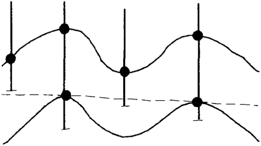
  Figure 6 Cross section showing two conformable surfaces. Dashed line represents direct modeling of lower surface data. Solid lines represent direct modeling of upper surface data and conformable modeling of lower surface data.

• 

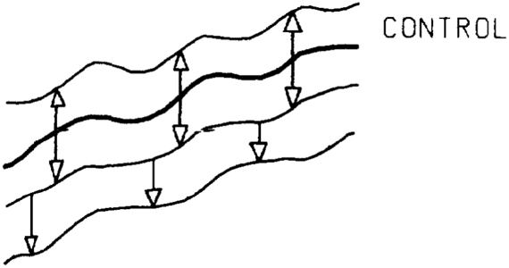
  Figure 7 Cross section showing four conformable surfaces. The second from the top is the control and is modeled using structure data. The other surfaces are built using the conformable method.

• 

  Figure 8 Cross sections showing that surfaces that intersect due to (a) baselap or (b) truncation will incorrectly cross one another.

• 

  Figure 9 Cross sections showing a baselapping surface (a) as coincident with the lower surface in areas of baselap (for cross section display) and (b) as missing in areas of baselap (for map display).

• 

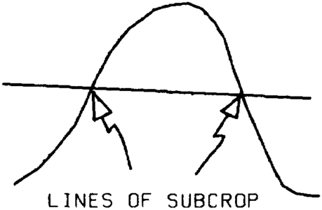
  Figure 10 Cross section showing surfaces before baselap operations. The zero contour of the model built by subtracting the two surfaces defines the subcrop line.

• 

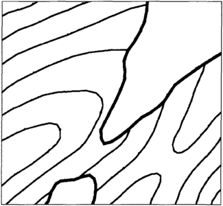
  Figure 11 Map showing contours and subcrop lines.

• 

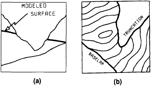
  Figure 12 The middle surface baselaps onto the lower surface and is truncated by the higher surface. (a) Cross section showing proper relationships. (b) Map showing surface contours and lines of baselap and truncation.

Conformity

A technique used to model conformable surfaces is thickness addition or subtraction. It is used because directly gridding each surface in a group of conformable surfaces may not produce the best results. Often variations in data distributions allow one surface to project past another or to have significantly more form definition than others of that sequence (Figure 6). The conformable technique builds a grid for the surface with the best data distribution (control surface) within a sequence of conformable surfaces and then adds or subtracts the adjacent interval's thickness to generate conformable surfaces above or below it. The newly constructed structural surface now becomes the surface to which thickness is added or subtracted to produce the next higher or lower surface. The process continues upward and downward until all surfaces within the sequence are constructed (Figure 7). This approach works well for complete data sets and vertical wells, although additional steps are required to handle deviated wells, partial penetrations, or missing data.

The conformable technique is often used to transfer the shape of an existing surface to a new surface while honoring the data of that new surface. Common applications include stream channels and the top of draping rock units.

Baselap and truncation

For computer mapping, the term baselap can be defined as the abrupt termination of a higher surface (usually depositional) against a lower surface. A similar definition could be used for truncation—the abrupt termination of a lower surface against a higher surface (usually an unconformity).

Most computer mapping systems build a surface model using only data for that surface. When one surface laps onto or truncates another, the initial surface models will almost always cross (Figure 8). This is expected and must be corrected. The following discussion describes methods for handling baselap and truncation in a grid-based mapping system.

Baselap

Baselap can be achieved in several ways. To baselap one grid onto another for the purpose of cross section display and volumetrics work, the elevation z values at each grid node are compared and the maximum value is retained in a new grid. This makes the two grids coincident in the area where the upper grid is missing due to base lap (Figure 9).

Contour maps of baselapping surfaces should have no contours in areas of baselap because the surface does not exist there. To baselap one grid onto another for map display, the elevation z values at each grid node are compared and the value of the baselapping grid is set to missing if lower or kept if higher than the other grid (Figure 9).

The subcrop line is the line of contact between a baselapping surface and the surface upon which it base laps (Figure 10). To generate this line, the elevation z values of one grid are subtracted from the other. The input grids must cross one another (grids before baselap) or the intersection cannot be established. The resulting intersection grid will have positive and negative values, and its zero contour will be the line of baselap.

To display contours and the subcrop line, contour the baselapped (blanked) surface grid and then on the same map draw only the zero contour from the intersection grid (Figure 11).

Truncation

With only a few modifications, the approach used for baselap can be applied to truncation. For cross section and volumetrics work, the two grids are compared and the minimum is kept as the new truncated grid. For contour display, the grids are compared and the values of the truncated grid are set to missing if higher or kept if lower than the other grid. The intersection grid for subcrop display is built just as it was for baselap.

Combining baselap, truncation, and conformity

In projects involving more than two surfaces, the techniques for baselap, truncation, and conformity are often used in combination (Figure 12). The following rules are used to order the techniques:

• On a hand-drawn cross section showing all surface relationships, identify the unconformities.
• Identify the sequences of conformable surfaces.
• Select a control surface (the surface that builds the best grid) for each sequence.
• Build grids for all unconformities and control surfaces.
• For each sequence, use the conformable technique to build all of the noncontrol grids.
• Starting with the lowermost surface, perform truncation and baselap operations, working up from the bottom.

Unique aspects of a project often require these procedures to be modified. However, the procedures provide a useful outline for getting started and guiding you through a project.

Faults

• 

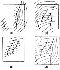
  Figure 13 Separate surface models are built for each fault block. (a, b, and c) The surface for each fault block is allowed to extend past faults defining the block edge. (d) When displayed, contours are constrained to inside the fault block polygon and all models are displayed on the same map.

• 

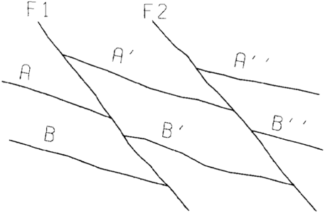
  Figure 14 Surface models are constructed for the faults and for each surface on each side of each fault. Operations between surface models prevent them from projecting past one another.

• 

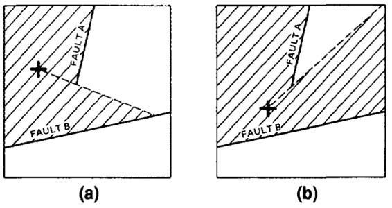
  Figure 15 Faults act as barriers beyond which data cannot be seen from the location for which a surface value is being calculated. (a) A grid node (indicated by +) to the west of fault A can only see data in the hatchured area. (b) A grid node farther to the south of fault A can see more data, thus the surface smoothly changes form around the fault ends.

• 

  Figure 16 (a) Surface model built with no fault constraints. (b) Model of vertical separation. (c) Unfaulted structure model built after removing vertical separation from data. (d) Faulted structure model built by subtracting separation model from unfaulted structure model.

• 

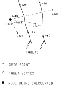
  Figure 17 The data value is adjusted by the separation of faults crossed by the line connecting the data point and the location for which an estimate is being made.

Few programs automatically identify faults based on input data; therefore, an interpretation of the presence and position of faults must be made prior to computer mapping. Once the fault interpretation has been made, several techniques exist for incorporating them into a surface model. Some commonly used methods are described here.

Fault block

The fault block or polygon technique uses polygons to isolate fault blocks. Typically, several sides of the enclosing polygon are faults, while some are lines (zero throw faults) used to close the polygon. Digitized contours and data points for the surface inside the polygons are used to build that fault block's surface model. A separate model is built for each of the surface's fault blocks. To create a contour map, each of the fault block surface models must be contoured separately with the contours constrained to stay within the fault block's polygon. All of the contours are drawn on the same map along with the fault traces (Figure 13). Similarly, volumes must be calculated on a block-by-block basis and summed for the unit.

Special care must be taken when constructing a fault block surface near sides of polygons that do not represent faults. Since these portions of the polygons have been drawn across unfaulted surfaces, grid node values should change smoothly across these polygon lines.

Fault gaps imply nonvertical faults, and traces with gaps would be expected to shift position from one surface to the next. Since digitizing polygons requires significant effort, the same set of polygons is often used for all surfaces (vertical faults). It is important to understand how a vertical assumption affects unit volumes.

Fault plane

The fault plane technique is used to model surfaces cut by nonvertical faults when enough data are available to model fault faces and structural surfaces on either side of those faults. Separate models are built for each surface on each side of each fault and for each fault plane. Baselap (maximum) and truncation (minimum) operations are used to prevent surface models from projecting through faults that bound them and to merge faults that intersect one another properly (Figure 14). The faults are treated as if they were unconformities and the surfaces between faults as if they were sequences, thus the previously described techniques apply. For more than a few faults (three or four), the ordering of the operations becomes complex. Both normal and reverse faults can be modeled.

If this technique is used, then creating displays and volumes for a surface or zone requires careful manipulation of a large number of surface models. This is because each surface is represented by a suite of surface models, one for each fault block. Also, much care is required to model surfaces cut by faults that fade out in the map area.

Fault trace

The fault trace technique uses fault trace locations and a faulted surface modeling algorithm to build continuous faulted surface models. The algorithm prevents data on one side of a fault from being used when assigning values to the surface model on the other side of the fault (line-of-sight method) (Figure 15). This technique is used by a large number of mapping programs.

For normal faults, the traces usually enclose an area called the fault gap. The gap represents the area where the structure surface is missing. Nodes in this area are typically set to missing, although they are sometimes assigned values representative of the fault plane. Traces that do not have gaps imply vertical faults and therefore will not change position from surface to surface. Traces for nonvertical faults should shift from surface to surface, and those for significant throws will show a gap in map view.

Contouring, cross section, volumetrics, and other surface display and manipulation algorithms must be modified to use fault traces. When modified, these algorithms do not use surface model values from one side of a fault for contouring and volume calculations on the other side of the fault.

Vertical separation

Surface-modeling algorithms that use a fault's vertical separation (see , for definition) can use data from one side of a fault when building a surface model on the other side of the same fault. This is because data on the opposite side of a fault are adjusted by that fault's separation before being used to calculate the surface's value.

Vertical separation modeling is usually handled either by (1) building a separation model for each fault and adjusting all the data at once or (2) adjusting each data point for vertical separation at the time it is used for surface modeling. In the first approach, a vertical separation model is built for each fault. All of the separation models for faults that affect a particular surface are added together. Data for that surface are shifted by the total separation at each location, moving them to their prefault position. A surface model is constructed using the adjusted data, and the total vertical separation model is then subtracted from the unfaulted surface model, creating the final faulted surface model (Figure 16).

The second approach is similar to the fault trace method in that it alters the use of a data point on the opposite side of a fault. However, instead of not using the point, it adjusts the point's z value by the vertical separation of the faults that lie between the point and the node being calculated (Figure 17).

Once constructed, cross sections, contour maps, volumes, and so on are commonly generated from these models using algorithms similar to those used for fault trace models. There are other methods for modeling with vertical separation, but regardless of which method is used, they all require significantly more information about faults than other fault-modeling methods. Often much of this information is not available. When this happens, most of these programs will “degenerate” to working as the fault trace method does.

Combined methods

Some programs blend two or more techniques together to produce faulted surface models. For example, one program blends the fault plane method with vertical separation modeling to produce a fault model that carries surface form across faults and properly migrates fault position with depth. Another program blends the fault plane method with the fault trace method to produce faults that properly migrate with depth.

Volumetrics

• 

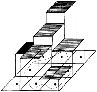
  Figure 18 The cell is centered on the grid node and lies either inside or outside the polygon. The cell's area is multiplied by its z value (thickness) and that volume is added to volumes for all other cells inside the polygon.

• 

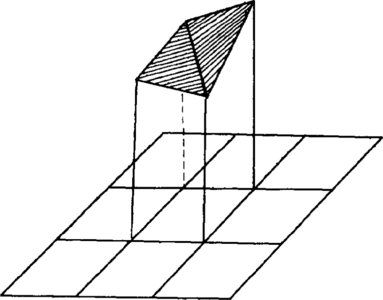
  Figure 19 The cell's corners are defined by grid nodes. The top is defined by two or more planes passing through the node z values and lie inside the polygon. The prism of volume under each plane is calculated and added to volumes for all other prisms inside the polygon.

• 

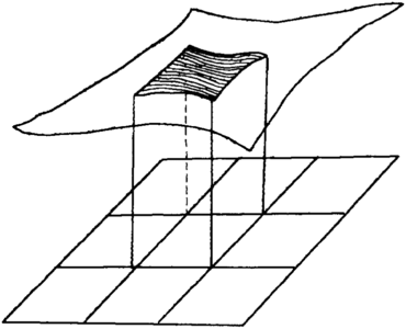
  Figure 20 A mathematical surface is fit to the grid cell. Calculus is used to integrate the volume under the curve, inside the grid cell, and inside the polygon. All cell volumes inside the polygon are added together.

• 

  Figure 21 Thickness Is normally defined by grids representing the top and base of reservoir and the fluid contact(s).

• 

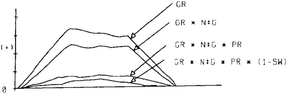
  Figure 22 The gross hydrocarbon rock thickness is progressively reduced by net to gross ratio, average porosity, and oil saturation, until only the thickness of pores filled with hydrocarbon remains.

• 

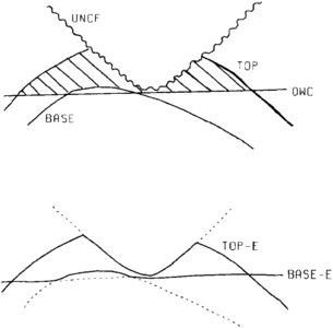
  Figure 23 The envelope technique is used to define one grid for the top of reservoir and another for the base of the reservoir. These are subtracted to create the gross hydrocarbon rock thickness.

• 

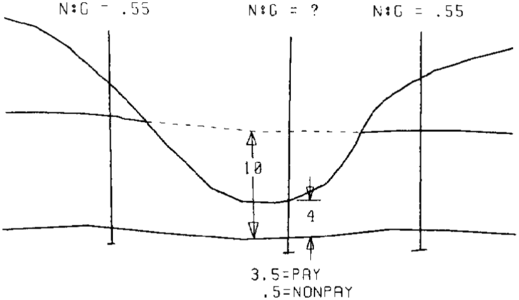
  Figure 24 Incomplete data for net and porosity due to partial penetrations, truncations, baselaps, and so on create problems when building models of these and related variables.

Estimates of volumes are normally calculated between two structure surfaces, above a fluid contact, or sometimes below another fluid contact.

The volumetrics algorithm

Following is a brief description of the range of volume calculation techniques used. This discussion uses a grid-based system, although similar procedures could apply to triangulated or other systems. The discussion assumes that volumes are calculated within a bounding area (polygon).

Volume by point count

Grid nodes will fall either inside or outside the polygon of interest. Statistics can be generated for the nodes that fall inside the polygon. Those statistics and the following equation are used to determine volume:

${\text{Number of nodes }}\times {\text{ Average value }}\times ~x{\text{-grid increment }}\times ~y{\text{-grid increment}}={\text{Volume inside the polygon}}$

This approach assumes that each grid cell extends from a base up to a flat top, which is the grid node's value, and that the node is in the center of the cell. If the center of the cell is inside the polygon, it is counted; if it is outside, it is not (Figure 18).

Volume by simple plane fits

Grid nodes occupy corners of grid cells, and a line is drawn diagonally across a cell dividing it into two triangles. The value at each corner of the triangle is known; therefore, a flat plane can be fit through these points. The base above which volumes are to be calculated is also a plane, and its value is known. Since the dimensions of the sides of the triangular prism are known from the grid increments, all of the information needed to calculate the prism's volume is available. The volume of all triangle prisms totally inside the polygon are calculated and summed. Any prisms partially within the polygon are subdivided into smaller prisms with the values at the corners of the smaller prisms linearly interpolated from the three original triangle corners. The volumes of these partial values are calculated, summed, and added to the volume of prisms totally within the polygon (Figure 19).

Volume by mathematical fit and integration

This approach integrates under a smooth mathematical surface passed through the grid nodes in and around the cell for which volumes are being calculated. As with the simple plane fit described previously, node values are at cell corners and volumes are calculated and summed for each cell and partial cell within the polygon. A common approach is to use 16 grid node values, 4 from the cell of interest and 12 from the adjacent cells. A third-order polynomial is fit to these 16 node values. By applying calculus to this polynomial over the area of the grid cell, the exact volume under the surface is determined (Figure 20). If only a portion of the cell is contained within the polygon, then the integration is performed only within that part of the cell.

Discontinuities and other constraints

Faults define surface discontinuities that must be accounted for if volumes are to be calculated accurately. A fault cuts a grid cell into two portions, each of which must have volumes calculated seperately. There are many approaches to doing this, all of them concerned with projecting the surface up to the fault in a reasonable manner. Each side of the fault is worked independently unless vertical separation is available; then a more sophisticated surface estimating approach can be used.

Political boundaries, porosity cutoffs, or other types of constraints must also be incorporated into the calculation. In some systems, these are incorporated into the model before going into the volumetrics program. In others, they are handeled automatically by the program.

Modeling and volume calculation in a thickness domain

A typical goal when preparing models for input to a volumetrics program is to create one model that represents the thickness of hydrocarbons (Figures 21 and 22). This is done by solving the following equation:

${\displaystyle {\mbox{HPT}}={\mbox{GR}}\times {\mbox{N:G}}\times {\mbox{PR}}\times (1-{\mbox{$SW}})} where

HPT = hydrocarbon pore thickness, which is a surface model representing the thickness of hydrocarbons. This is integrated over the area of interest to determine hydrocarbon pore volume (HPV).
GR = gross hydrocarbon rock thickness, which is a surface model representing total thickness of the interval containing hydrocarbons.
N:G = net to gross ratio, which is a model or constant representing the ratio of porous (pay) rock thickness to gross rock thickness.
PR = average porosity, which is a model or constant representing the average porosity of the porous rock.
SW = water saturation, which is a model or constant representing the average water saturation.

There are many considerations when building each of these surface models.

Building the GR model

To build a surface model for the gross hydrocarbon rock thickness (GR), we envelope the volume of interest by building one surface model for its top and another for its base. These surface models should cross where the volume goes to zero.

The top of volume model is built by comparing all surface models that define part of the top of volume envelope (top-E), creating a single model that is the minimum of their values. Next, compare all surface models that define part of the base of volume envelope (base-E) and create a single model that is the maximum of their values (Figure 23).

Once constructed, the base of volume model is subtracted from the top of volume model, creating the gross rock thickness model. This model is positive where thickness exists and either zero or negative where it does not. The negatives in this case are desired as they allow clear definition of the reservoir edge (zero line).

Other variables for volumetrics

Often porosity and water saturation (and sometimes net to gross ratio) are input as constants representing the average value over the area of interest. Otherwise the variables are entered as surface models. Creating these surface models is complex and can be done in many ways. One of the most common is to digitize a hand-drawn map and build a model. Another is to build a model from well data. During model construction and use, certain issues must be considered:

• Incomplete information caused by partial penetration, eroded top, faulting, and so on is often encountered. When this happens, the value of net to gross ratio or any other parameter being modeled will only represent the portion of the rock unit present. Figure 24 demonstrates this problem for a partially penetrating well. The N: G for the middle well is 0.875 (or 3.5/4), while for the left and right wells, which fully penetrate the unit, the N: G is 0.55. Clearly the partial unit value does not correctly represent the “true” unit value. If the missing portion was pay, then the N: G would be 0.95 [(3.5 + 6)/10]. If the missing portion was nonpay, then the N: G would be 0.35 (3.5/10). The true N: G lies somewhere between these two limits. Special techniques must be used to model incomplete data.
• Modeling water saturation using standard algorithms and well data generally does not produce acceptable results. This is because the amount of water in the oil or gas portion of the reservoir is dependent upon porosity, permeability, height above fluid contact, and other factors. Generally several engineering functions (J-curves) that relate porosity, height above fluid contact, and water saturation are used to convert structure top, structure base, fluid contact, and porosity models to a water saturation model. The resulting model can be adjusted to honor the existing water saturation data at wells.
• Net to gross and sometimes average porosity can change rapidly in the area extending from the point where the base of reservoir encounters the fluid contact to the reservoir edge (wedge zone). If the vertical distribution of net rock is not homogeneous throughout the reservoir, then these variables may change significantly in the wedge zone relative to values where the reservoir is full thickness. Often these changes are ignored. Sometimes the reservoir is separated into subzones, with a full suite of volumetric models constructed for each subzone. Three-dimensional modeling of net and porosity is a more precise solution.
• If more than one of the four models input to the HPT equation contain negative values, then additional incorrect volumes could result. This is because these models are multiplied together, and if two have negative values at the same location, the resulting value will be positive, creating a volume where no volume should exist. A commonly used safety measure is to clip porosity, water saturation, and net-to-gross models to a minimum value of zero, eliminating the problem. Zeros in the model often produce a very jagged zero line contour. However, that is preferred rather than significant volume errors. There are techniques for correcting these jagged zero contour lines.

Modeling and volume calculation in a structure domain

Some programs calculate volumes directly from structure surface models. This has several advantages, two being simpler input and the ability to define horizontal levels above and below which volumes should be calculated. If this type of program allows only one surface for the top and one for the base of volume, then the same techniques for enveloping the volume described previously must be used. How the porosity, N: G, and water saturation grids are used may vary from program to program and must be understood for one to have confidence in the results.

Other surface modeling tools

In addition to algorithms for gridding, contouring, and cross section display, there are many other tools required for effective computer mapping. Whether a grid, triangulated mesh, or other surface model is used, most of these tools are needed. Where appropriate, the term surface model is used instead of grid to make the descriptions more general. Here is a list of some of those tools:

• Single data and surface operations—Add, subtract, multiply, and divide by a constant, trigonometric functions, blank max, blank min, clip max, clip min, normalize, dip and azimuth, statistics, rotate, and so on.
• Dual data and surface operations—Add, subtract, multiply, divide, union, intersection, max, min, blank max, blank min, clip max, clip min, and so on.
• Polygon blanking—One or more polygons are used to blank or set to another value data or surface values inside or outside the polygons.
• Merge data—Combine two data files by concatenation, union, or intersection.
• Range subset data—Select a range of acceptable values for one or more data fields and build a subset of the original data set that fits within those ranges.
• Resample grid—Given an old grid and a new arrangement of grid nodes (due to changes in origin, x-y limits, or x-y grid increments), calculate z values for the new grid using surrounding node values from the old grid.
• Grid to data—Convert a grid to data.
• Back interpolate—Given x-y locations from a data file, calculate z values at those locations from a surface model. Either create a new field in that data file, replace all of an existing field, or replace missing values in an existing field.
• Filter surface model—Smooth a surface model while either honoring or not honoring a given set of data. Optionally use a variety of constraints to limit how the filter is applied or the area over which it is applied.
• Volumetrics—Calculate volumes below a surface model (isochore), above a plane, and within a polygon. Optionally calculate volumes between two or several surface models and within a polygon.

See also

• Cross section
• A development geology workstation
• Log analysis applications
• Introduction to contouring geological data with a computer
• Two-dimensional geophysical workstation interpretation: generic problems and solutions

External links

find literature about Using and improving surface models built by computer

• Original content in Datapages
• Find the book in the AAPG Store

salt water