Pressure transient testing

Development Geology Reference Manual
Series	Methods in Exploration
Part	Production engineering methods
Chapter	Pressure transient testing
Author	W. John Lee
Link	Web page
Store	AAPG Store

Pressure drawdown and buildup tests

Information derived from tests

Pressure buildup and drawdown tests provide an opportunity to obtain estimates of the following well and reservoir properties:

• Permeability to the produced phase (oil, gas, or water), which is an average value within the radius of investigation achieved in the test
• Skin factor, which is a quantitative measure of damage or stimulation in the well
• Current average pressure in the drainage area of the tested well
• Verification of flow barriers (such as faults) and estimates of distance to these barriers

Single-rate flow tests

A single-rate flow test is run using the following procedure. Start with the reservoir at a uniform, stabilized pressure. Then place the pressure measuring device as near the perforations as possible. Flow the well at a strictly constant rate (control with a variable choke or other control device). An alternative method for gas wells is to measure surface pressures and calculate bottomhole pressures from surface measurements. The rate at which pressure changes with time reflects the formation properties. An example of this type of test is a single-point deliverability test in a gas well (see Production testing).

Pressure buildup tests

In a pressure buildup test, one should stabilize the rate in the tested well for several days, that is, maintain the rate approximately constant. Then place a pressure measuring device as near the perforations as possible several hours before shut-in. Shut the well in and let the pressure build up. The rate at which pressure builds up with time reflects the formation properties. (For more details of pressure buildup and flow tests, see Matthews and Russell.)

Multi-rate flow tests

These tests are run much like single-rate tests, except that the rate is changed by discrete amounts one or more times while the test continues. An example of this type of test is a flow after flow deliverability test on a gas well, which is also called a four-point or back-pressure test.

When the tests are applicable

Flow tests can be useful when the reservoir is at uniform pressure, such as when a new well is completed or when a well has been shut in for a lengthy period. Flow tests are appropriate when a well must continue to produce revenue even though a test is needed. Analysis of flow tests is simplest when the rate is held strictly constant and in all cases requires known rates at all times during the test.

Buildup tests are appropriate at virtually any time in the life of a well because they simply require that the well be shut in. Buildup tests have the advantage that the rate (zero) is much more easily controlled than in a “constant rate” flow test. For this reason, buildup tests are overwhelmingly the preferred type of pressure transient test in practice.

How the tests are analyzed

• 

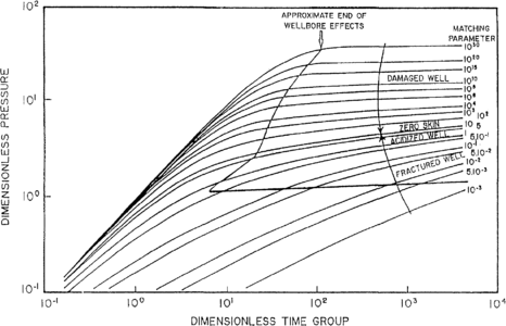
  Figure 1 Type curve that identifies the end of wellbore effects.

• 

  Figure 2 (a) Derivative type curve used to match derivatives of test data. (b) Shapes of derivatives of test data for various reservoir conditions.

• 

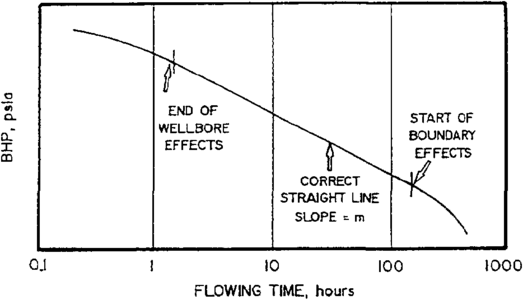
  Figure 3 Typical flow test data graph.

• 

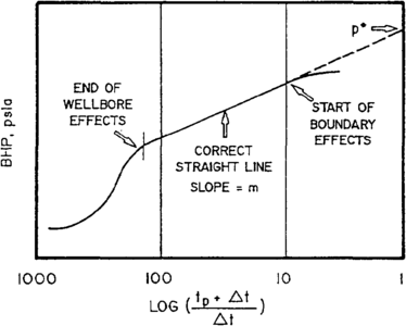
  Figure 4 Typical buildup test graph (Horner plot).

• 

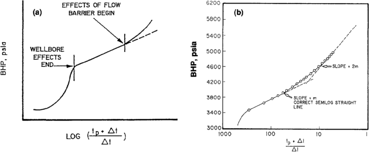
  Figure 5 (a) Typical buildup curve shape with flow barrier, (b) Doubling of slope on Horner plot for well near barrier.

Wellbore effects dominate early test data. The end of wellbore effects is found using log-log plots of test data, which are compared to preplotted type curves, as illustrated in Figure 1. The shapes of test data plots are also used to identify the reservoir type, such as homogeneous acting, naturally fractured, layered, or hydraulically fractured. Derivative type curves (basically the slope of a plot of pressure versus the logarithm of time) are particularly helpful for identifying reservoir type and wellbore effects, as shown in Figures 2(a) and (b).

Traditional analysis is focused on semi-logarithmic plots of test data, with slopes of straight lines on these plots used to determine permeability. Figure 3 is a typical semi-log plot of flow test data, and Figure 4 is a typical semi-log plot of buildup test data. The “correct” semi-log straight line is indicated on these figures; the line is identified with the help of type curves (see Production histories). On the buildup test plot, shut-in bottomhole pressure is plotted versus the logarithm of the ratio of producing time, t_p, plus shut-in time, Δt, to shut-in time. This plot is called a Horner plot, named for the person who proposed it in the petroleum literature.

Simple equations allow us to estimate permeability and skin factor once the correct semilog straight line is identified and its slope, m, is estimated. These equations apply to both drawdown and buildup tests. The following equations are used for oil wells:

$k={\frac {162.6qB\mu }{mh}}$

and

$s=1.151\left[{\frac {\Delta p_{1{\rm {hr}}}}{m}}-\log \left({\frac {k}{\phi \mu c_{\rm {t}}r_{\rm {w}}^{2}}}\right)+3.23\right]$

where

• k = effective permeability to produced phase (md)
• q = flow rate (STB/day)
• B = formation volume factor (rb/STB)
• m = slope of semi-log straight line (psi/log_10cycle)
• h = net pay thickness (ft)
• s = skin factor (dimensionless)
• Δp_lhr = pressure change in first hour of test (psi)
• ϕ = porosity (fraction)
• μ = viscosity (cp)
• c_t = total compressibility of formation and its fluids (psi^–1)
• r_w = wellbore radius or hole size (ft)

Similar equations are used for gas well test analysis.

Extrapolation of pressure in a buildup test to Horner time ratio of unity provides an estimate of original reservoir pressure (new well) or “false” pressure, which serves as the basis for determining current drainage area pressure, ${\bar {p}}$, for a well with some pressure depletion in its drainage area caused by extended production of fluids. Figure 4 illustrates extrapolation of pressure to time ratio of unity.

Also, distance to boundaries of flow barriers is found from semilog plots by deviation from a previously established semilog straight line. In the simplest case, which is uncommon except for wells very close to boundaries, the late time slope doubles. Figure 5(a) shows the usual case, where the slope increases at late times but does not double. Figure 5(b) shows the less common case where the slope actually doubles at late times. The time at which the deviation occurs and the amount of deviation can be used to estimate the distance from the tested well to the flow barrier.

Long-term production tests

• 

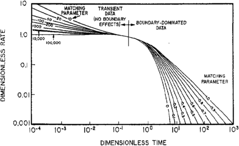
  Figure 6 Fetkovich's type curve for analyzing long-term production data. After Fetkovich.

• 

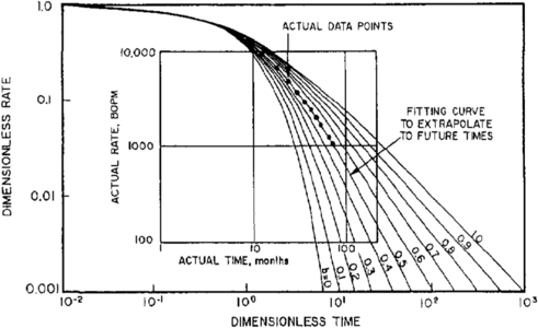
  Figure 7 Actual production data matched on a Fetkovich type curve.

• 

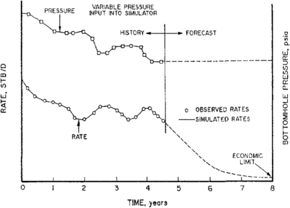
  Figure 8 History match of production data and forecast of future performance.

The same information is available from long-term production tests as from short-term flow tests, including permeability, skin factor, and distance to boundaries. Hydrocarbons in place in the tested well's drainage area can frequently be estimated from these test data. Once boundaries have affected the test data, long-term production data can be extrapolated to provide a forecast of future production to the economic limit and can thus provide a reserve estimate for the well.

How the tests are run

These are not tests in a formal sense. The rate is simply monitored as a function of time while the well is produced at an approximately constant bottomhole pressure (BHP). If constant BHP cannot be maintained, one should at least measure surface pressures continuously (from which one attempts to calculate the variable BHPs).

These “tests” are applicable at any time. The data are most readily analyzable if the well is produced at approximately constant BHP or when BHP and flow rate are known continuously as functions of time.

How the tests are analyzed

The simplest of these tests—those with production data from wells produced at constant BHP or with smoothly changing rates and BHP—can be analyzed with simple type curves, such as Fetkovich's, illustrated in Figure 6. Formation properties are obtained from matches of actual field data to the type curve. Forecasts are made by projecting future performance along the type curve that matches post-production performance.

An essential requirement in this method of analysis is that there is enough production history for boundary effects to have influenced production data. This same requirement also applies to conventional decline curves and decline curve analysis—if boundary effects have not been felt, the decline curve projection is totally meaningless and certainly incorrect. Figure 7 shows a type curve match of past performance and indicates how production data can be extrapolated into the future.

More complex tests, with abrupt changes in rate and BHP, are more readily analyzed with computer reservoir simulators. These simulators are used to history-match production data to obtain a reservoir description, which is then used to obtain a long-term production forecast and thus to estimate reserves. Figure 8 shows an example of a history match of production data and a forecast of future performance of the well using the reservoir description obtained from the history match.

Interference and pulse tests

Figure 9 Active and observation wells in an interference pulse test.

Interference and pulse tests are run to obtain the following information:

• Whether tested well pairs are in pressure communication
• Directional permeabilities between tested well pairs
• Average porosities in the areas influenced by the tests

How the tests are run

• 

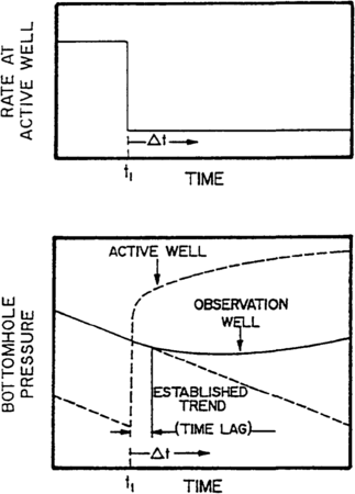
  Figure 10 Schematic illustration of rate history and pressure response for an interference test. (After .)

• 

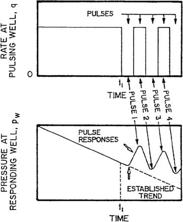
  Figure 11 Schematic Illustration of rate (pulse) history and pressure response for a pulse test.

Interference tests are run by first shutting in the portion of the reservoir in the area affected by the test. Then one produces (or injects into) one well (called the active well) and measures the pressure response in the offset wells. Figure 9 shows a typical interference test pattern, and Figure 10 is a plot of a typical response in an observation well.

Pulse tests are performed by first producing (or injecting into) the active well for a few hours. The active well is then shut-in, then returned to production, shut-in again, and so on in a regular, repeating pattern. The response in the offset wells is then measured while continuing to produce all wells in the field except those directly involved in the test. This is possible because the “noise” caused by continued production of wells not directly involved in the test can be filtered out using the response caused by the repeated on-off pattern in the active well. Figure 11 shows a typical response in a pulse test observation well.

Comparison of pulse and interference tests

Interference tests are usually much more expensive than pulse tests because of the loss of revenue arising from having to shut-in a major portion or all of the tested reservoir to conduct the test. Also, ambiguity exists in interference test interpretation because it is uncertain that an observed response was actually caused by the active well. In a pulse test, if a repeated signal is received in an observation well, there is little doubt that it was caused by the rate changes in the active well.

When the tests are applicable

Interference and pulse tests are applicable whenever one needs to know whether two or more wells in a formation are in pressure communication. They are also used in improved recovery processes (water, gas, or other fluid injection projects) in which knowledge of directional permeability differences and reservoir description generally are critical to the success of the project.

These tests work best in formations that have higher permeabilities, closer spacing, and single-phase flow. In gas reservoirs, high formation pressure is more desirable than low pressure in achieving a successful test.

How the tests are analyzed

Simple tests in homogeneous-acting, isotropic or anisotropic, infinite-acting (that is, no boundary effects during the test), single-layer reservoirs can be analyzed with readily available interpretation charts and type curves. Most actual tests require computer reservoir history-matching for analysis because of heterogeneities, boundaries, and layers.

See also

• Production testing
• Production histories
• Artificial lift
• Surface production equipment
• Stimulation
• Introduction to production engineering methods
• Well completions
• Production logging
• Production problems
• Workovers

External links

find literature about Pressure transient testing

• Original content in Datapages
• Find the book in the AAPG Store
• Dictionary:Pressure transient testing in Sheriff's Encyclopedic Dictionary

stock tank barrels

bottom hole pressure