Reservoir modeling for simulation purposes

Development Geology Reference Manual
Series	Methods in Exploration
Part	Reservoir engineering methods
Chapter	Reservoir modeling for simulation purposes
Author	Koen Weber
Link	Web page
Store	AAPG Store

Fluid flow in a reservoir is controlled by bed continuity, the presence of baffles to flow, and the permeability distribution (see Fluid flow fundamentals). Reservoir heterogeneities influencing fluid flow range from large scale faults and discontinuities down to thin shale intercalations, sedimentary structures, and even pore scale features (Figure 1).

Figure 1 Classification of reservoir heterogeneity types.

Simulation studies (see Conducting a reservoir simulation study: an overview) performed at early stages of field development are done to estimate parameters such as optimal well spacing, while at later stages the objectives may be infill drilling or secondary recovery. The role of the geologist is to provide reservoir models that give a sufficient description of those parameters that control the fluid flow relevant to the planned simulation study. The key to effective and economic field development planning lies in early recognition of those reservoir characteristics that control drive mechanisms, sweep efficiency, and consequently, well spacing requirements and possible need for pressure support. The significance of the various heterogeneity types for oil recovery is summarized in Table 1, where • denotes a strong effect, and × a moderate effect.

Table 1 Significance of reservoir heterogeneity type for oil recovery

Reservoir heterogeneity type	Reservoir continuity	Sweep efficiency		ROS in swept zones	Rock-fluid interactions
		Horizontal	Vertical
Sealing fault	•	•
Semi-sealing fault	×	•	•
Nonsealing fault	×	•	•
Boundaries as genetic units	•	•	•
Permeability zonation within genetic units		×	•	×
Baffles within genetic units		×	•	×
Laminations, cross-bedding		×	×	•
Microscopic heterogeneity				•	×
Textural types				•	•
Mineralogy					•
Tight fracturing		×		•
Open fracturing		•	•	•

The steps in the modeling process are as follows:

• Determining the facies of the reservoir rock through data gathering from cores and logs
• Rock typing for each environment of deposition to estimate permeability from log derived porosity and estimation of vertical permeability
• Correlation of all wells to provide a framework for the delineation of a simulation model
• Determination of an optimal grid block pattern using the flow unit principle
• Mapping the reservoir properties in each grid block layer

Data gathering

The realism and reliability of the resulting model is a function of the reservoir heterogeneity but also of the planning that has gone into the data gathering. Defining suitable data gathering schemes for a specific field requires multidisciplinary cooperation and a sound understanding of the significance of the data. Analog cases and sensitivity studies on prototype models can guide this process which is crucial to the reliability of the results. In Table 2, an overview is given of the value of the different types of data for the identification and quantification of reservoir heterogeneities. Only a part of the data are of geological nature. Reliable information on reservoir connectivity is often derived from production and pressure tests (see Production testing and Pressure transient testing). In particular, it is very difficult to determine large scale vertical permeability from core and log data.

Table 2 Value of data for identification and quantification of reservoir heterogeneities

Reservoir heterogeneity type	Detailed seismic	Reservoir pressure		Production data/tests					Well logging			Rock sample		Outcrop or analog reservoir
		Horizontal distribution	Vertical distribution	Production tests	Pulse tests	Tracer tests	Production history	Production logs	Standard	Special	ROS	Cores	SWS cuttings
Sealing fault	•	•	×	×	•	×	•		•	×	×	×		×
Semi-sealing fault	•	•	×	×	×	×	×		•			×		×
Nonsealing fault	•	×	×						•			×		×
Boundaries as genetic units	×	•	•	×	×	×	×	×	•	×	×	•	×	•
Permeability zonation within genetic units			×	×	×			×	•	•	•	•	×	•
Baffles within genetic units			×		×		×	×	•	×		•		•
Laminations, cross-bedding										×		•		•
Microscopic heterogeneity, textural types, mineralogy										×	×	•	×	×
Tight fracturing				•			•					•		×
Open fracturing	×	•	×	•	•	×	•	•	×			•	×	×

The detail to which a reservoir can be modeled is a function of both the degree of heterogeneity and the data density. At an early stage of development, one may be restricted to seismic data, sparse well data, and production tests only. In these circumstances, we reap maximum benefit from knowledge of the typical flow characteristics associated with the prevailing facies and diagenetic overprint and of a data base to predict reservoir body continuity and architecture. Regional experience in analog fields can often be used to guide the modeling process.

The data that form the basis for reservoir modeling ideally comprise regional data, seismic data, cores, logs, pressure measurements, wireline formation tests, pulse tests, and well-planned production tests (Table 2). Modern three-dimensional seismic data can be used for a range of modeling purposes from structural analysis to reservoir properties such as thickness, lithology, porosity, and pore fill (also see Geophysical methods).

The effect of large scale features such as faults can be estimated on the basis of geological experience and modeling or it must be evaluated by pressure measurements or fluid level differences.

Rock typing and permeability estimation

• 

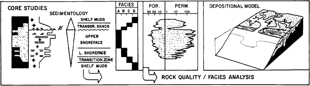
  Figure 2 Analysis of core data for facies identification and rock quality assessment.

• 

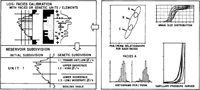
  Figure 3 Log-facies calibration and determination of facies-related rock characteristics.

The first priority in describing the reservoir rock is the determination of the environment of deposition and the range of lithofacies that occur within the reservoir (see Lithofacies and environmental analysis of clastic depositional systems and Carbonate reservoir models: facies, diagenesis, and flow characterization). Regional stratigraphic information, cores, and sidewall samples are used for this purpose. Of particular interest is the rock typing through a study of porosity, permeability, petrography, and capillary properties (Figure 2) (see Laboratory methods). For simulation purposes, permeability is a major parameter, and estimating the permeability profile in noncored wells is of prime importance. The basis for these techniques is multivariate analysis of the combined logging data. Discriminant analysis of log response using a core calibrated system usually leads to the best results. In general, one has to combine several rock types into an electrofacies class mainly because of the poor vertical resolution of the nuclear logs if run in standard fashion. If the porosity and permeability relationships of combined rock classes differ little, this is an acceptable simplification (Figure 3).

Well correlation

Figure 4 Correlation of reservoir units and subdivision of reservoir In flow units.

The next step in reservoir modeling is correlating the reservoir intervals from well to well (Figure 4). This procedure is strongly dependent on facies and well spacing. A requirement is a sound database of genetic unit geometry, for example, width to thickness ratio of a specific sand body type. When no deterministic correlation can be made of reservoir units, it may be necessary to use probabilistic modeling techniques, but in such cases only prototype simulations are usually carried out.

The framework for constructing simulation models is controlled by facies distribution, major permeability contrasts, and impermeable layers. Again, maximum use should be made of reservoir engineering data with emphasis on wireline formation pressures. Geological predictions of sealing surfaces are often unreliable because of the presence of small scale faults or local erosion.

Grid block patterns

The reservoir has to be subdivided in such a way that all major baffles are represented and that the individual layers and bodies can be described using average petrophysical properties that lead to realistic flow simulations. For this purpose, the term flow unit has been introduced, which is defined as a volume of rock characterized by a specific combination of geological and petrophysical properties that influence fluid flow (see Flow units for reservoir characterization). Flow units can be composed of a combination of stratigraphic elements if they do not essentially differ in fluid flow criteria.

The subdivision of the reservoir into flow units is typically a multidisdplinary activity because geological and reservoir engineering information has to be used together. Economic considerations with respect to numbers of grid blocks to be used also play a role.

Reservoir simulation operates on the principle of simultaneously solving the flow equations between adjacent blocks of rock in response to offtake from wells. The larger the number of grid blocks used, the closer the model resembles the geological prototype. However, even with the fastest computers, the simulation models are restricted to a maximum of some 60,000 grid blocks. For economic reasons, most simulations make use of less than 10,000 grid blocks. Consequently, grid block sizes normally range from 100 to length::300 m in diameter and from 5 to length::15 m in thickness (see Conducting a reservoir simulation study: an overview).

Practical grid block sizes usually imply the amalgamation of a few geological features. Thus, an averaging procedure is required to obtain realistic overall flow characteristics for the blocks as a whole. The influence of discontinuous shale breaks on vertical permeability, for example, can be estimated using a statistic approach. Averaging horizontal and vertical permeability over grid block size units is a difficult task. In practice, the effective horizontal permeability usually ranges from the arithmetic to the geometric average of the permeability profile of the block. The more continuous the sublayers of the flow unit, the closer the average is to the arithmetic average. The more random the permeability, the closer it gets to the geometric average. Geostatistical methods have become popular to tackle these problems. Vertical permeabilities are difficult to measure, and the values used are often based either on experience for a given facies or on vertical pulse tests or other pressure data evaluation.

Mapping of reservoir properties

Figure 5 Mapping of reservoir properties per grid block layer to provide input for the reservoir simulation.

The geological input to three-dimensional reservoir simulation must consist of structural maps and property maps. Typically, maps must be prepared for every simulation model layer, specifying the distribution of net/gross, isochores, porosity, horizontal and vertical permeability, capillary pressure curve characteristics, and water saturation (Figure 5). Also, the geologist and the reservoir engineer have to cooperate to define pseudo-relative permeability curves for different internal grid block heterogeneity types. The matching phase of the simulation study requires similar cooperation to arrive at a final model with realistic properties.

Modeling carbonate reservoirs

Modeling of carbonate reservoirs is generally more difficult than modeling clastic reservoirs. The reason is that carbonate rocks usually undergo a much more complex pattern of diagenetic processes. As a result, the permeability distribution can be complex and poorly related to original facies distribution. A further complication can be the occurrence of open fractures.

Carbonate reservoirs without fractures can in principle be treated similarly to clastic reservoirs. Reservoir simulation of so-called dual porosity reservoirs is difficult because of the problem of quantifying the degree of capillary contact across fractures. Recently, methods have been proposed to tackle the problem of block-to-block interaction. In all cases, carbonate reservoirs require a considerable amount of core studies and frequent use of the scanning electron microscope and its auxiliary equipment.

See also

• Enhanced oil recovery
• Drive mechanisms and recovery
• Reserves estimation
• Waterflooding
• Fluid flow fundamentals
• Conducting a reservoir simulation study: an overview
• Introduction to reservoir engineering methods
• Petroleum reservoir fluid properties

External links

find literature about Reservoir modeling for simulation purposes

• Original content in Datapages
• Find the book in the AAPG Store

References

- ↑ Harris, D. G., 1975, The role of geology in reservoir simulation studies: Journal of Petroleum Technology, May, p. 625–632.
- ↑ WEBER
- ↑ Hurst, A., Archer, J. S., 1986, Sandstone reservoir description—an overview of the role of geology and mineralogy: Clay Minerals, v. 21, p. 791–809., 10., 1180/claymin
- ↑ 5.0 5.1 Slatt, R. M., Hopkins, G. L., 1990, Scaling geologic reservoir description to engineering needs: Journal of Petroleum Technology, Feb., p. 202–210.
- ↑ Ruijtenberg, P. A., Buchanan, R., Marke, P. A. B., 1990, Three-dimensional data improve reservoir mapping: Journal of Petroleum Technology, Jan., p. 22–61.
- ↑ Weber, K. J., Mandl, G., Pilaar, W. F., Lehner, F., Precious, R. G., 1978, The role of faults in hydrocarbon migration and trapping in Nigerian growth fault structures: Offshore Technical Conference, Houston, OTC 3356.
- ↑ Wolf, M., Pelissier-Combescure, J., 1982, Faciolog-automatic electrofacies determination: SPWLA Third Annual Logging Symposium Transactions, July.
- ↑ Haldorsen, H. H., Brand, P. J., Macdonald, C. J., 1987, Review of the stochastic nature of reservoirs: Proceedings of the Seminar on Mathematics of Oil Production, Cambridge, U., K.
- ↑ Weber, K. J., Van Geuns, L. C., 1990, Framework for constructing clastic reservoir simulation models: Journal of Petroleum Technology, Oct., p. 1248–1297.
- ↑ Begg, S. H., Chang, D. M., Haldorsen, H. H., 1985, A simple statistical method for calculating the effective vertical permeability of a reservoir containing discontinuous shales: Society of Petroleum Engineers Symposium on Reservoir Simulation, Dallas, TX, Feb. 10–13, SPE 14271.
- ↑ Journel, A. G., Alabert, F. G., 1990, New method for reservoir mapping: Journal of Petroleum Technology, Feb., p. 212–218.
- ↑ Por, G. J., 1989, A fractured reservoir simulator capable of modelling block/block interaction: SPE Annual Technical Conference and Exhibition, San Antonio, TX, Oct. 8–11, SPE 19807.