Reservoir simulation study

This article describes the steps necessary to conduct a detailed reservoir simulation study (also see Reservoir modeling for simulation purposes). A simulation study requires description of the reservoir's rock and fluid properties, validation of completion and production history, and extensive history matching to validate and modify this input data. When history matching is complete, numerous predictions of field and well performance characteristics are calculated for various development scenarios.

The reservoir characterization required to define porosity and permeability for each grid block in a reservoir simulation model is more stringent and at the same time more loosely defined than reservoir characterization required in detailed development geology studies. A simulation engineer can spend countless hours defining the reservoir model. Nevertheless, despite the plausibility of the interpretation used to develop this description, the ultimate test of the simulation model's validity is its reproduction of production data. The smaller relative uncertainty of production data with regard to input data dictates that simulation engineers may take many liberties in matching that data, while rationalizing their choices with a broad degree of latitude. Development geologists are the most likely source of quality control for the reservoir description developed and modified for a reservoir simulation study.

Model specification

Figure 1 Typical models used in reservoir simulation. (a) Zero-dimensional tank. (b) One-dimensional linear. (c) One-dimensional radial. (d) Two-dimensional cross-sectional. (e) Two-dimensional area. (f) Two-dimensional radial. (g) Three-dimensional. From Mattax and Dalton, © 1990 Society of Petroleum Engineers.

A simulation study begins by choosing a model type from among those shown in Figure 1. A grid, which determines the resolution at which the complex reservoir flow equations are solved, is then selected. The model's size is defined by the number of grid blocks resulting from the grid overlain on the field or field segment being studied. In general, the accuracy of results from simulation studies is greater for smaller grid block sizes. Smaller grid block sizes permit more detailed descriptions of reservoir heterogeneity and more accurate resolution of fluid fronts and phase behavior. An optimum grid size is often determined by running test cases at several different grid sizes. The largest grid size at which no appreciable change in the results occurs is selected for the study.

Practical limits on the size of reservoir simulation models are often imposed by computational expense or capabilities. These constraints may dictate that the size of the reservoir segment being simulated must be reduced or the grid block size increased. Simulating small characteristic segments of a field using a fine grid may be preferable to simulating larger segments using a coarse grid. Small models can provide insight into the mechanics of production performance (such as viscous flow, gravity, or heterogeneity). For example, a fluid injection project can be studied using detailed areal and vertical models rather than a coarse grid three-dimensional model. Extrapolating results from these mechanistic models to field performance can be accomplished using their results to modify general recovery characteristics defined by coarse grid models.

Preparing fluid properties

Two types of fluid descriptions are used in reservoir simulation studies: black oil and compositional. The black oil description expresses the fluid's volumetric (formation volume factor and solution gas-oil ratio) and flow (viscosity) characteristics as a function of pressure for three phases: oil, gas, and water. In complex fluid mixtures, the fluid's volatility often dictates that volumetric and flow characteristics are not only a function of pressure but also of composition. For these fluids, a compositional description uses an equation of state to describe the fluids' volumetric and flow characteristics. An equation of state describes a fluid in terms of the fundamental physical properties of its components: methane, ethane, heptanes-plus, and so on. These fundamental physical properties—critical pressure, critical temperature, critical volume, acentric factor, and interaction coefficients—are unique for each compositional fluid description derived for a simulation study.

Black oil fluid descriptions are used to describe most oil and gas fields. Primary depletion, waterflooding, and gas injection can all be simulated with black oil models. Volatile oil reservoirs or gas condensate reservoirs generally require compositional models. These models may exhibit such complexities as a fluid whose density is linearly proportional to depth or whose phase switches repeatedly between oil and gas. Thermal models, used to simulate steam injection, may use either black oil or compositional fluid descriptions. Black oil thermal models describe fluid properties as a function of temperature as well as pressure. The importance of oil volatilization in thermal recovery often dictates that compositional models are used to simulate thermal recovery processes.

Preparing multiphase flow properties

Figure 2 (a) Pseudo-relative permeability and (b) capillary pressure curves calculated for two-layer thicknesses compared to laboratory measurements. (From Coats,, after Mattax & Dalton, © 1967, 1990 Society of Petroleum Engineers.)

Fluid saturations and the produced fractions of oil, gas, and water are determined by capillary pressures and relative permeabilities specified as functions of water saturation. Equilibrium (initial) fluid saturations are directly dependent on capillary pressure, which is itself a function of height above the fluid contacts, the fluid densities, porosities, permeabilities, and the surface chemistry of the fluids. Once production or injection commences, fluid movement is controlled by the relative permeability of each phase (except at very low velocities where the effects of capillary pressure are important). In a reservoir consisting of two fluid phases, oil-water, gas-oil, or gas-water capillary pressures and relative permeabilities must be specified. For a three-phase system, relative permeabilities and capillary pressures for two of the three possible systems are specified.

Capillary pressure may be expressed using the Leverett J-function. This function can be used to calculate capillary pressure as a function of each grid block's porosity and permeability. Sufficient data may also exist to correlate relative permeability curves' initial and residual saturations with porosity. Rather than assign individual capillary pressure and relative permeability curves for each grid block, average curves can be derived for several ranges of porosity and permeability values (also referred to as regions).

Relative permeability and capillary pressures characterizing grid blocks may differ considerably from laboratory measurements. Laboratory measurements minimize the effects of gravity and heterogeneity. An example of these pseudo-relative permeabilities and capillary pressures is shown in Figure 2. The importance of gravity and heterogeneity effects is greater with larger layers. Pseudo-relative permeability and capillary pressure curves are often developed on small detailed studies for larger scale models. In some cases, pseudo-relative permeability and capillary pressure is developed during history matching. Pseudo-relative permeability and capillary pressure may be dependent on fluid and saturation history. Their ability to account correctly for gravity and heterogeneity is limited. Where these effects are significant, a smaller grid size should be used.

Preparing matrix properties

• 

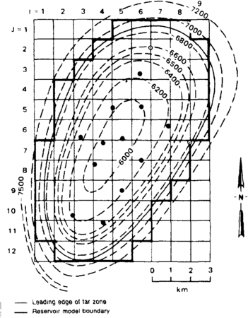
  Figure 3 Model grid overlain on Khursaniyah field, Saudi Arabia. (From Boberg, © 1974 Society of Petroleum Engineers.)

• 

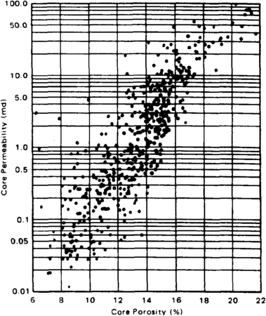
  Figure 4 Core measurements from the Bradford Sandstone. (From Levorsen.)

• 

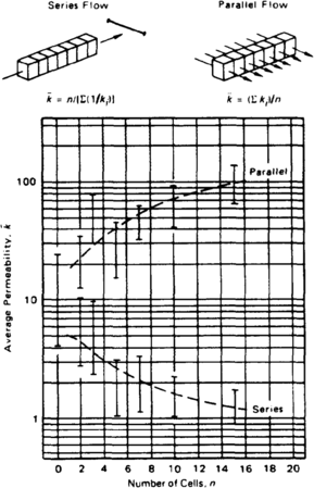
  Figure 5 Comparison of mean permeabilities calculated for series flow (geometric average) and parallel flow (arithmetic average). © Lishman, Courtesy Canadian Institute of Mining, Metallurgy, and Petroleum.

Matrix properties describe reservoir characteristics specified at each point of the grid (matrix) overlying the reservoir model (Figure 3). Once a grid has been selected, the average depth, thickness, porosity, and permeability are calculated for each grid block. Digitized structure and isopach maps may be used with mapping and gridding software to calculate average depths and thicknesses. Mapping software is used to convert the digitized contour maps to an interpolated grid of values. The mapping grid should be several times finer than the reservoir simulation grid since the values in the mapping grid falling within grid block boundaries are used to calculate the depths and thicknesses for each grid block. If the mapping grids are fine enough, a simple averaging of the values within each grid block will suffice to calculate their values corresponding to the grid block centers.

Porosities are calculated for each grid block in a method similar to that described for reservoir depths and thicknesses. First, the porosities calculated at 0.5- to 1-ft intervals from well logs must be averaged for each simulator layer. These layer porosities are then contoured and gridded. More advanced techniques for calculating three-dimensional porosity distributions (such as stochastic and geostatistical methods) are topics of current research, but they are beyond the scope of this chapter. The porosity values for each grid block are calculated by averaging the porosity grid values that lie within the boundaries of each grid block.

Permeability is often correlated as a function of porosity (Figure 4). The porosities calculated at 0.5- to 1-ft intervals from well logs are used to calculate horizontal and vertical permeabilities for the same intervals. Permeability averaging techniques require special consideration. For porosity, a volumetric averaging technique produces the same volume of void space for the averaged block as exists in all the smaller blocks. For permeability, averaging techniques must ensure that the flow rates of the averaged blocks are the same as the combined flow rates of the smaller blocks. Arithmetic averaging is used to calculate the average horizontal permeability at the well for each simulator layer. Geometric averaging is used to calculate the average vertical permeability. These layer permeabilities are then contoured and gridded. Figure 5 shows that the choice of permeability averaging technique has a significant effect on the calculated average.

Initializing the model

The first step in any model study is the calculation of pressures and fluid saturations before the onset of production. At this point in time, the model should be in static equilibrium. Distinct fluid contacts should appear at the appropriate depths, and the potential (the sum of pressure and the gravity head) should be equal everywhere in the model. A model that exhibits indistinct fluid contacts or uneven potentials (meaning that flow will occur in the next time step without production) has not been initialized properly.

History matching

Figure 6 Simulated water production for Initial and modified reservoir description. (From Mattax & Dalton, © 1990 Society of Petroleum Engineers.)

Reservoir simulation models are normally calibrated using production history. During this process, significant modifications to the reservoir description may be required to match historical performance. Figure 6 shows the initial trial and the final match achieved in a well model. History matching is often a trial-and-error process requiring 20 model runs or more before a satisfactory match between the predicted and observed performance is realized. In new fields, little data exists and reservoir performance predictions may be made without history matching, but this produces unreliable performance predictions. Any data at all, even well tests from discovery and delineation wells, should be used to calibrate the reservoir model. Because of the relatively minuscule volume of data sampled by well logs, it is simple to construct a model that produces performance predictions that diverge dramatically from actual results. Any amount of data, unless it has been proven erroneous, is more credible than performance predictions from the most elaborately constructed simulator.

History matching is usually conducted by using the production data to specify the production rate for one phase, either oil or gas. With this phase specified, the model calculates the rates of the other phases. History matching attempts to match the rates of the unspecified phases and any pressure measurements.

Modifications in reservoir description needed to match history are rarely straightforward. Pressure decline is a function of initial fluid volume, the rate of fluid production, and fluid properties. The rate of fluid production is a function of the drainage area pressure, the permeability of the formation and close to the well, relative permeabilities, and fluid properties. A discrepancy between observed and calculated pressures can be caused by an incorrect pore volume, incorrect interwell permeabilities that allow too little or too great fluid recharge after production, or incorrect relative permeabilities resulting in the incorrect rate of production for the second producing phase. Failure to model larger scale features properly, such as interlayer communication, aquifer support, or faults, may also be responsible for discrepancies in pressure matches. Discrepancies in predicted rates can be equally as difficult to match. Wellbore conditions may also have a significant effect on history matching.

History matching continues to be an art. Even final matches are subject to uncertainty since the large number of parameters that can affect the results precludes identification of a single unique match. The participation of a geologist in the modifications to reservoir description that occur during history matching can greatly enhance the possibility that the final description will approximate the actual reservoir.

Predicting performance

Predictions almost always begin by calculating the projected performance of the base case. The base case represents the mode of operations where everything remains exactly as it stands on the last day of the history match. In its strictest interpretation, the base case means no new wells, recompletions, workovers, or changes in a well's artificial lift status. In practice, the base case means these changes usually occur to the extent that they could have been foreseen (they are already in the budget or 5-year plan) or by extrapolating today's producing (or injecting) rules into the future (any well producing below a certain rate is converted to gas lift).

Each prediction case must specify each well's producing rules. The location of each well to be produced or injected during the prediction must be specified, including the time at which it is considered active. In the simplest case, wells are constrained to produce at a constant rate or at a constant bottomhole pressure. Economic limits can also be specified. Using simple rules, the simulator output must be run in increments of 1 year or less so that the results can be scanned to determine whether changes should be made in a well's status, completion, or constraints to reflect the field's operating practices. This process is time consuming since the simulator must be constantly monitored and rerun.

Advanced simulators have tremendous flexibility with regard to producing rules. Operating constraints imposed by gas plants can be simulated by specifying a constant group rate. Water plant constraints can be simulated by specifying a maximum water rate. Gas lift injection or pumping can be simulated by calculating well rates using bottomhole pressures derived from wellbore gradient calculations and by allocating the total amount of gas lift gas or electricity to each well based on its productivity. Plug backs can be simulated by automatically recompleting producing grid blocks when saturations exceed a specified value in the initial grid block. Wells can be drilled to maintain a specified target rate by searching for high saturation grid blocks. These are just a few of the many special features that can be used to simulate producing rules.

See also

• Enhanced oil recovery
• Drive mechanisms and recovery
• Reservoir modeling for simulation purposes
• Reserves estimation
• Waterflooding
• Fluid flow fundamentals
• Introduction to reservoir engineering methods
• Petroleum reservoir fluid properties

External links

find literature about Reservoir simulation study

• Original content in Datapages
• Find the book in the AAPG Store

References

- ↑ 1.0 1.1 1.2 Mattax, C. C., Dalton, R. L., 1990, Reservoir simulation: Richardson, TX, Society of Petroleum Engineers.
- ↑ Coats, K. H., 1967, Simulation of three-dimensional, two-phase flow in oil and gas reservoirs: Society of Petroleum Engineers Journal, Dec., p. 377–388; Transactions, AIME, v. 240.
- ↑ Boberg, T. C., 1974, Application of inverse simulation to a complex multireservoir system: Journal of Petroleum Technology, July, p. 801–808; Transactions, AIME, v. 257.
- ↑ Levorsen, A. I., 1967, Geology of petroleum, 2nd ed.: San Francisco, W. H. Freeman Publishing, p. 128–129.
- ↑ Lishman, J. R., 1970, Core permeability anisotropy: Journal of Canadian Petroleum Technology, April-June, p. 79-84.