Seismic data - mapping with two-dimensional data

Mapping two-way time

Most two-dimensional seismic reflection lines are presented in the format of horizontal distance versus two-way traveltime (time sections). Using interpreted time sections and a geographic base map, one can draft structure contour maps.

Preparation for mapping

Before mapping, double-check that variations in the frequency, phase, and (especially) polarity of wavelets were accounted for during interpretation. Lines that were processed differently may appear to correlate well, even though they actually do not. Also, make sure that the interpreted events tie at the intersections between lines. You may construct a map perfectly, but if the lines are misinterpreted, your map will be misleading (see Seismic interpretation).

The basemap should have clearly legible line and shotpoint numbers. The shotpoints should be printed at intervals that are smaller than the wavelength of the structures that will be mapped. The base map should be printed accurately, but sometimes mistakes occur. Remember that the accuracy of the base map partly determines the accuracy of your geological interpretation. If you question the accuracy of any part of the base map, consult with the person who drafted the map or check the field records yourself.

Recording times of events

Begin mapping by recording the two-way times of the event being mapped for every shotpoint along each line and for all line intersections. The precision of time picks will vary with the scales of lines, but be as precise as possible. The numbers that are recorded are raw times. It is advisable that the times be recorded on a rough draft base map and in tabular form.

In some cases, the distances between the shotpoints printed on the lines are too large for resolving relatively small structures. In this case, it might be necessary to interpolate a ground position and then record a time. However, be aware that a relative position between two shotpoints on a line may not correspond to the same relative position between the same two shotpoints on the basemap. In short, the only ground positions that you can locate accurately on the base map are those that are printed on the base map. If highly accurate intermediate ground positions are important for your interpretation, refer to the person who drafted the map for help or check the field records yourself.

Misties

• 

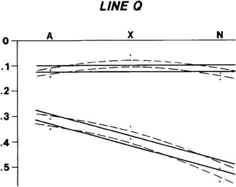
  Figure 1 False structure (dashed lines) created when misties are averaged. Dots show times of events on seismic lines A, X, and N where those lines intersect line Q. Solid lines show true attitude of beds. If dashed events were mapped, false structure would appear.

• 

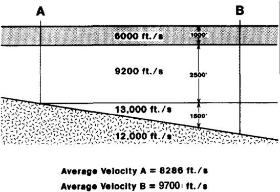
  Figure 2 (a) Crude base map illustrating seismic line intersections. (b) Table showing misties at seismic line intersections (times in milliseconds). Circled lines constitute a group having small misties. A group can be used as a base to which times on all other lines are adjusted. For example, times on line A561–80 could be shifted down about 52 msec.

Usually, raw times do not match perfectly at the intersections between two lines. These differences in time are known as misties, and can range in magnitude from 1 msec to tenths of 1 sec. Misties often result between lines that are processed differently, particularly when different datums are chosen for the statics routine. Small misties may also result because normal migration routines cannot compensate perfectly for the geometry of dipping events. Commonly, misties result from “end-of-line” effect, where one line crosses the poorly migrated end of another line. Misties can also arise from errors in the interpretation or in the reading of two-way time.

Misties are corrected mathematically. Differences of a few milliseconds are normally small enough that they can be averaged. However, when the differences approach the magnitude of the structures that you want to resolve, they must be treated by other methods. Averaging large misties (“splitting the difference”) is ill-advised because doing so may introduce nonexistent structures to your map (Figure 1).

In general, adjusting for large misties in a group of lines starts by identifying a subgroup with very small misties. This subgroup is used as a base to which the times of events on all other Unes are adjusted (Figure 2). Adjustments are made by shifting all the times of all the events on a given line by the same amount. Properly honoring the data requires that, for a given line, all the times for every event be adjusted by a constant value (Figure 2). For example, do not adjust one event up 5 msec and another 15 msec on the same Une; this would introduce more time (i.e., depth) between the two events.

The end result after adjusting for misties will not be perfect. In cases where scores of lines are being used, some of the final misties may actually be quite large. However, the object is to minimize the error, which is an attainable goal.

Contouring

After the misties are adjusted, the revised two-way times can be plotted on the final base map. Finally, the points can be contoured at an interval that you deem appropriate.

Other types of maps

• 

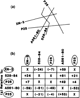
  Figure 3 Illustration showing effect of lateral differences in velocity on conversion of time and depth. If a single velocity function of 8300 ft/sec were used, errors of +6 ft at A and -440 ft at B would appear on the depth map.

• 

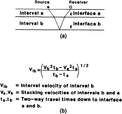
  Figure 4 (a) Illustration of ray paths, intervals, and interfaces used to help explain the Dix formula. (b) The Dix formula for calculating interval velocities, which assumes that interfaces are flat and smooth.

• 

  Figure 5 Velocity map with velocities marked at grid intersections.

• 

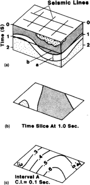
  Figure 6 (a) Block diagram showing the time that Is mapped for a time slice map. (b) Interval that is mapped on time interval map. (c) Time interval map.

Velocity gradient maps

A velocity gradient map is constructed at an intermediate step between a time map and a depth map. During conversion from time to depth, a velocity gradient map compensates for lateral changes in velocity, which is preferable to using a single velocity function (Figure 3). Construction requires a base map and velocity data. The object is to contour the average velocity down to an event.

Velocity data generally come from five sources: vertical seismic profiles (VSPs), checkshot surveys, synthetic seismograms, stacking velocities, and well depth to time correlations. The latter is an easy and reliable method of determining velocities. Simply match the time of a horizon on a seismic line with the depth of that horizon in an adjacent well and you can calculate a velocity. This method may not work in highly deformed rocks, in which one is unsure exactly what the two-dimensional seismic line is imaging. However, depth to time correlations generally work well.

Vertical seismic profiles and checkshot surveys are also excellent sources because they show the actual traveltime of sound through material over a known distance, thereby yielding true velocities. Good estimates of velocities are provided by synthetic seismograms. Synthetics are made from sonic logs and show the cumulative travel time through the rocks where a sonic log was run. Knowing the cumulative travel time for a given depth, one can calculate a velocity (distance divided by time).

Approximate velocities can be calculated using the stacking velocities that were picked during processing (Figure 4). This is the poorest source of velocity information, but it may be the only source in areas where no wells have been drilled. Stacking velocities are usually printed at the top of each seismic line. Use the nearest shotpoint printed under the stacking velocities as the “ground position” for your calculated average velocities. Keep in mind that stacking velocities are not true velocities; they are just the velocities that the processor interpreted as the best at tuning events during processing. Occasionally, these velocities can vary from true velocities by more than 20%. However, they generally approximate the root mean square velocities from which average velocities can be calculated.

Depth maps

Basically, depth maps are constructed by multiplying a one-way time map by a velocity gradient map. Hence, the times on a two-way map must be halved before this calculation takes place. A basic map can be made by simply multiplying one-way time by velocity at every point where velocity data exist and then contouring the products. A much better result is obtained by gridding both the time and velocity maps (Figure 5) and then multiplying the time by the velocity at each grid point. Both grids can be constructed by interpolating values between points where data are available. After multiplying time by velocity at each grid point, contour the products. The gridding method is easily done with a computer and mapping software.

Time interval maps

Time interval (or isotime or isochron) maps are commonly used for interpreting changes in thickness between interpreted horizons (Figure 6). To map time intervals, calculate the difference in time (normally two-way time) between two events at each shotpoint and contour the resultant values.

Time slice maps

A time slice map shows geology in the horizontal plane at a given time (normally two-way time) (Figure 6). In essence, making a time slice map is analogous to making geological maps from cross sections. As a first step toward construction, imagine that all the data above your chosen time disappear and that your base map lies directly on top of the chosen time. Next, locate each intersection between an interpreted event and the chosen time and plot that intersection at the ground position immediately above. Finally, link the points for each respective event in a manner that is consistent with your knowledge of the structure on the lines.

Computer-aided mapping

Interpretations derived from seismic lines can be mapped efficiently with the help of a computer workstation, which performs repetitive calculations very quickly. First, the interpretations must be entered into a workstation, either by interactive (on-screen) interpretation or by digitizing interpretations that exist on printed lines. Mistie corrections are then performed by the computer. Two-way times and time intervals can then be posted on a base map. Contouring time and time interval maps can be done by the workstation, but the result usually requires some hand editing (see A development geology workstation).

Constructing depth maps is possible once hand-drawn time and velocity maps are digitized into the workstation. The computer grids and multiplies the time and velocity maps, and the resultant values can then be contoured.

See also

• Three-dimensional seismic method
• Seismic interpretation
• Synthetic seismogram
• Vertical and lateral seismic resolution and attenuation
• Forward modeling of seismic data
• Displaying seismic data

External links

find literature about Seismic data - mapping with two-dimensional data

• Original content in Datapages
• Find the book in the AAPG Store

References

- ↑ Tucker, P. M., Yorston, H. J., 1973, Pitfalls in Seismic interpretation: Tulsa, OK, Society of Exploration Geophysicists Monograph Series n. 2, 50 p.
- ↑ Dix, C. H., 1955, Seismic velocities from surface measurements: Geophysics, v. 20, p. 68–86, DOI: 10.1190/1.1438126.