Seismic inversion

	Development Geology Reference Manual
Series	Methods in Exploration
Part	Geophysical methods
Chapter	Seismic inversion
Author	Brian Russell
Link	Web page
Store	AAPG Store

The object of seismic inversion is to convert the seismic interpreter's view of the earth reflections as a function of time to the geologist's view of the earth velocity as a function of depth. This is not as easy as it may seem. The reason for this is that seismic data measurements are taken at the earth's surface and involve sending a sound pulse through the earth and recording the echoes from each reflecting interface. The farther this sound pulse has to travel, the more the pulse is distorted and the less information it is able to carry back to the surface. Obviously, drilling a well and running a set of logging tools gives us much more information. However, the advantage of the seismic method is that coverage can be made over large areas of the earth's surface. This is especially true of the large three-dimensional surveys that are now routinely being acquired. For this reason, seismic inversion is an important processing tool.

Seismic inversion methods

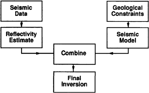
Figure 1 A flowchart showing the general concept behind seismic Inversion.
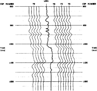
Figure 2 Band-limited inversion of several traces around a reef. The integrated sonic log from the reef well is shown as the dark trace in the central part of the figure.
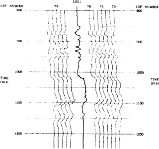
Figure 3 Model-based inversion of several traces from around a reef. The integrated sonic log from the reef well is shown as the dark trace in the central part of the figure.

As just mentioned, seismic data give us a “fuzzy” picture of the subsurface over a large area, whereas wells give us detailed geological information at a few points. This suggests a general approach to the seismic inversion method, as shown in Figure 1. On the left side of this flowchart, the input is our best reflectivity estimate from the seismic data. On the right side, we introduce geological constraints taken from a sonic log or seismic velocity information and produce a forward model. We then combine the information from the seismic data with controlling information from the seismic model and produce a final inversion result.

There are two main types of inversion currently being used. The first is band-limited inversion, which involves directly integrating the seismic trace. Since the seismic trace lacks a low frequency velocity trend because of the band-limited wavelet, the inverted trace lacks the “excursions” seen on the original sonic log. We must therefore add in the low frequency component from the geological model. The result is a frequency band-limited version of the original sonic logs. This is shown in Figure 2 for a carbonate reef example. The heavy trace in the center is a sonic log from the producing well. The zone of interest is at 1150 msec.

The second type of inversion, which is more recent than the band-limited method, involves producing a “blocky” output rather than a band-limited output. There are several methods that produce this type of output, and they are sometimes referred to as sparse-spike or model-based methods. These methods work by producing a forward model that best reproduces the seismic data when converted to synthetic form (that is, when the reflection coefficients are convolved with the wavelet). This method involves starting with a simple “guess” of this model and changing this guess iteratively until the error between the model and the observed seismic data is minimized (see Forward modeling of seismic data). The results of doing such a model-based inversion are shown in Figure 3 for the same traces shown in Figure 2. Notice that the carbonate reef is visible, and looks like the blocked version of the log.

Three-dimensional case study

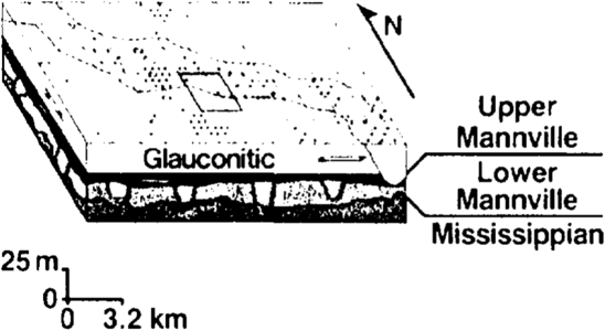
Figure 4 A schematic diagram of a river channel zone. Copyright: the Taber area of southern Alberta. The 3-D survey was done in the area outlined by the rectangle in the center of the map. Courtesy of Western Geophysical.
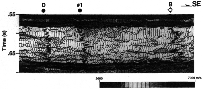
Figure 5 The model-based inversion of the line through the river channel system of Figure 4. Copyright: Western Geophysical.
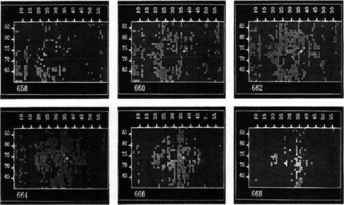
Figure 6 Time slice displays through the 3-D survey of the river channel zone. The lightly shaded areas show low velocity material in which reservoir sands are present. Copyright: Western Geophysical.

As an example of inversion applied to real data, let's consider a 3-D case study that was done in the Taber area of southern Alberta, Canada, by Western Geophysical. Figure 4 shows a schematic interpretation of the geology of a river channel zone. The area of interest is the Glauconitic Formation of the lower Cretaceous upper Mannville Group, which is characterized by rapidly changing lithological facies. The reservoirs are sandstones with porosities of 15% surrounded by impermeable siltstone.

A 3-D survey measuring 2.2 by length::1.7 km was acquired, as indicated by the rectangle in Figure 4. These data were then processed through to final migrated stack, and the result was inverted using the SLIM inversion method of Western Geophysical. This approach is similar to the model-based algorithm discussed earlier. The results of inverting one particular line from the 3-D volume are shown in Figure 5. Two producing wells and one dry hole are shown in this line. The producing interval is between 640 and 660 msec on the two producers, whereas the low velocity zone on the dry hole comes from a sand that is porous but not prospective. Figure 6 shows a series of time slices (that is, horizontal cuts through the 3-D data volume at constant time intervals) over the complete dataset (see Seismic data - mapping with two-dimensional data). Borehole B from Figure 5, which was the dry hole, is indicated by the faint white crosshairs at the centers of the graphs in Figure 6. The lightly shaded areas show areas of low velocity material at the zone of interest. Notice that this well is obviously mispositioned with respect to the low velocity reservoir material.

Conclusions

In this brief summary of inversion methods, we have considered two different approaches: band-limited and model-based. Band-limited inversion is a robust method that produces a smooth and continuous output. Model-based inversion produces a blocky output that contains more geological detail than band-limited inversion. However, both methods can be useful in the delineation of hydrocarbon reservoirs.

External links

find literature about
Seismic inversion

Seismic inversion

Contents