Seismic migration
| Development Geology Reference Manual | |

| |
| Series | Methods in Exploration |
|---|---|
| Part | Geophysical methods |
| Chapter | Seismic migration |
| Author | Ken Lamer, David Hale |
| Link | Web page |
| Store | AAPG Store |
Virtually all seismic data processing is aimed at imaging the earth's subsurface, that is, obtaining a picture of subsurface structure from the seismic waves recorded at the earth's surface. Deconvolution, for example, aims to sharpen reflections, and common midpoint (CMP) stacking exploits data redundancy to enhance signal-to-noise ratio while producing a seismic time section that simulates what would have been recorded in a zero-offset seismic survey, that is, one in which a single receiver, located at each seismic source position, records data generated by the source at that position.
Of the many processes applied to seismic data, seismic migration is the one most directly associated with the notion of imaging. Until the migration step, seismic data are merely recorded traces of echoes, waves that have been reflected from anomalies in the subsurface. In its simplest form, then, seismic migration is the process that converts information as a function of recording time to features in subsurface depth. Rather than simply stretching the vertical axes of seismic sections from a time scale to a depth scale, migration aims to put features in their proper positions in space, laterally as well as vertically.
All the issues in seismic migration reviewed here are treated in the collection of reprints found in Gardner.[1]
What migration accomplishes
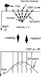
Figure 1 Schematic depth section (top) and zero-offset time section (bottom) for a single boulder at depth.
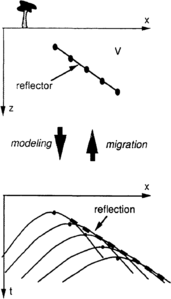
Figure 2 Schematic depth section (top) and zero offset time section (bottom) for a dipping reflector at depth.
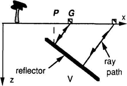
Figure 3 Schematic depth section showing normal incidence ray paths for two-way travel between source-receiver positions and a dipping reflector.
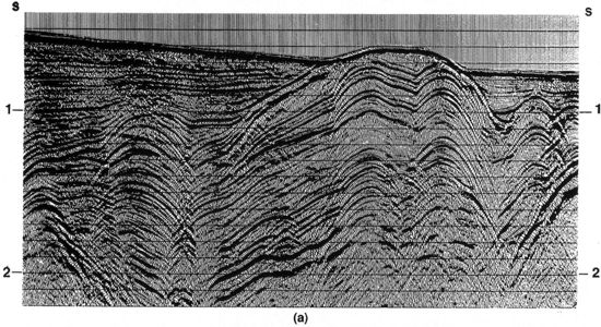
Figure 4a CMP stack of data from the Santa Barbara Channel, offshore California.
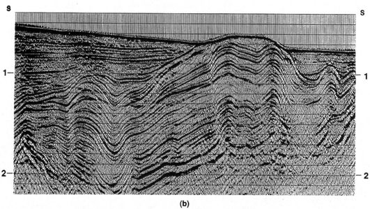
Figure 4b Result of migration.


The migration problem is illustrated in Figure 1. The upper part of the figure depicts a zero-offset survey conducted over a subsurface medium that is homogeneous (constant P-wave velocity) with the exception of an isolated boulder at some depth. Also shown are the straight ray paths traveled by seismic waves from each of five different source positions down to the boulder and back up to receivers located at the sources. Clearly, reflections from the boulder will be observed at all the surface locations, not just the one directly above it. Also, the reflection time clearly increases as the source-receiver pair is moved farther from the point directly above the boulder. The bottom part of Figure 1 shows schematically the seismic section that would be obtained for this survey. Reflections occur along a hyperbolic diffraction pattern with the apex at the same CMP location as that of the boulder.
The task of migration here is to convert or map reflections along the diffraction into a single point at the position of the boulder. The reverse process, by which the boulder gives rise to the observed diffraction pattern, is called modeling.
While the earth's subsurface is more complicated than that shown in Figure 1, the seismic data that would be obtained over the real earth can for all purposes be represented as a superposition of many diffraction curves generated by each of many boulder-like anomalies in the subsurface.
Figure 2 shows another depth section and associated seismic section for a subsurface consisting of a single dipping reflector. For a constant-velocity subsurface, the many weak diffractions from very closely spaced points along the reflector (of which five are shown in the figure) give rise, through constructive and destructive interference, to a net reflection along the straight-line envelope of the diffraction curves. Note that the reflection is displaced laterally from the true reflector position (the line connecting apexes of the diffraction curves). It is this lateral mispositioning of reflections from dipping reflectors that gave rise to the term migration for the process that corrects the positioning.
Figure 3 shows another perspective on this mispositioning. Reflections recorded at zero source-receiver offset follow ray paths that are perpendicular to the reflector. As a result, the reflection from the point on the reflector beneath point P, for example, would be recorded by the geophone at location G, to the right.
Figure 4 shows the application of migration to CMP-stacked field data. The superposition of diffraction curves evident in the unmigrated data of Figure 4a gives rise to crossing reflections that can not plausibly be interpreted as structure. By correcting for lateral mispositioning of dipping reflectors and collapsing diffraction curves to zones defined by the diffraction apex, migration converts the recorded waves to a subsurface picture (Figure 4b) depicting both broadly and tightly folded anticlines and synclines.
How migration is accomplished
One senses the massive scale of the computer intensive two-dimensional mapping involved in the transformation from unmigrated to migrated data in Figure 4. While these schematic sections depict what migration aims to accomplish, they say little about how it is done. All of the many methods of doing migration are founded on solutions to the scalar wave equation, a partial differential equation that models how waves propagate in the earth. A simple form of the wave equation is as follows:

where P(x, z, t) is the seismic amplitude as a function of reflection time t at any position (x, z) in the subsurface, and V is the seismic wave velocity in the subsurface, a function of both x and z. Disturbances initiated by a seismic energy source are assumed to propagate in accordance with solutions to the wave equation. Migration, then, involves a running of the wave equation backward in time, starting with the measured waves at the earth's surface P(x, z = 0, t), in effect pushing the waves backward and downward to their reflecting locations.
All current computer-based approaches to migration involve this backward solution to the wave equation. The earliest form, Kirchhoff summation migration, intuitively follows the situation depicted in Figure 1. In essence, recorded amplitudes on CMP traces are summed along the diffraction trajectories dictated by the assumed subsurface velocity distribution, and the sums are placed at the apexes of the curves, one curve for each sample point in the output migrated section.
Finite difference migration numerically integrates the wave equation by the method of finite differences to push seismic waves backward into the subsurface. A third category of migration approaches is f-k migration, which operates via Fourier transforms in the frequency wavenumber (f-k) domain. In general, Fourier transform methods provide elegant means of solving partial differential equations. When applied to migration, this elegance is often complemented by high computational efficiency.
Each of the different approaches has specific advantages such as computational efficiency, accuracy for imaging steep reflectors, and accuracy in the presence of spatial variation of velocity. Likewise, each can produce undesirable processing artifacts related to some limitation in data quality such as poor signal to noise ratio, too coarse a spatial sampling interval, and missing data (e.g., due to seismic source misfires).
Velocity: the key parameter
Regardless of the migration approach implemented, the key parameter of the process is velocity. Since migration involves pushing waves back to their reflecting points, it is essential that the waves be pushed backward through the same medium through which they have propagated. Clearly, waves will not get back to the correct position at a given time if the velocity used in the migration process differs from the actual subsurface velocity. Unfortunately, subsurface velocity is seldom well known, particularly in geologically complex areas. Today's migration algorithms are highly accurate when supplied with the correct subsurface velocity. Because subsurface velocity can only be estimated, however, migration yields only an estimate of the true subsurface.
Where lateral variation of velocity is modest (as in many places in the Gulf of Mexico), migration methods in the class called time migration have performed adequately. Where lateral velocity variation is severe (as in many overthrust areas), more computationally intensive depth migration is required. Note that the terms depth and time migration do not relate to whether the migrated results are presented as a function of time or depth. Results of both migration categories are most often displayed in time (as in the examples shown here) because of added uncertainties in results converted to depth. While depth migration is capable of accurate subsurface imaging where velocity is complex, the required accurate estimation of velocity is difficult and time consuming.
Poststack versus prestack migration
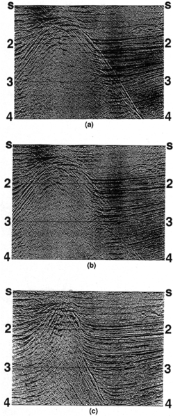
Figure 5 (a) CMP stack showing reffections from a salt dome in the Gulf of Mexico. (b) Stack after DMO processing. Steep portions of diffractions and reflections are now preserved. (c) Migration of the DMO-processed data shows the steep flank of the salt dome to be a particularly strong reflector.
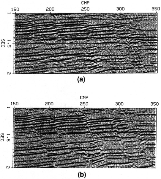
Figure 6 (a) Unmigrated and (b) migrated stack of DMO-processed data from the Gulf of Mexico.


While migration algorithms are capable of accurately imaging reflections from steep interfaces, shortcomings in CMP stacking lead to destruction of such reflections before conventional poststack migration is applied. Two alternatives to poststack migration of CMP stacked data preserve reflections from steep interfaces. Migration can be applied to the unstacked data (so-called prestack migration) so that the data need not be reduced to an approximation to zero offset before migration. The improvement in imaging of steep reflectors by this approach, however, is bought at the price of a great increase in the amount of computation required for the migration.
A cost-effective and accurate alternative to full prestack migration is to apply poststack migration to data that have had the added step of dip moveout (DMO) applied after normal moveout (NMO) correction, but before the data are stacked. DMO, a form of partial prestack migration, completes the process that NMO only imperfectly accomplishes—it converts data recorded with separated sources and receivers to a close approximation to zero-offset data, preserving reflections from both gently dipping and steep reflectors. Figure 5 shows the improvement in imaging of the steep flank of a salt dome achieved by poststack migration when applied to DMO-processed data.
The additional accuracy of either DMO or prestack migration over that of conventional poststack migration demands special care in the field acquisition of seismic data. Too coarse a spatial sampling, that is, too large a geophone group interval, may preclude high resolution imaging of steep reflectors by any migration method.
The example in Figure 6 shows imaging of reflections from steep faults. While migration of CMP-stacked data (not shown here) shows the faulting, reflections from the faults themselves are absent. Details of the fault reflections seen on the DMO-processed result can be diagnostic of sealing along the faults.
The schematic diagrams shown here have been two-dimensional (2-D) representations, and the illustrations have all involved 2-D migration of 2-D seismic data. Invariably, the earth's subsurface has three-dimensional (3-D) complexity. As a result, the mispositioning of recorded reflections extends in two lateral directions, and migration must be done as a 3-D process (see Three-dimensional seismic method for Reservoir Development). It suffices here to state that migration is fundamentally incomplete unless it is applied as a 3-D process to 3-D data.
See also
References
- ↑ Gardner, G. H. F., ed., 1985, Migration of Seismic Data: Tulsa, OK, Society of Exploration Geophysicists Monograph Series, 462 p.
External links
| find literature about Seismic migration |