Seismic processing basics

	Development Geology Reference Manual
Series	Methods in Exploration
Part	Geophysical methods
Chapter	Basic seismic processing
Author	Peter M. Duncan
Link	Web page
Store	AAPG Store

The printable version is no longer supported and may have rendering errors. Please update your browser bookmarks and please use the default browser print function instead.

The seismic data written to tape in the dog house, whether on land or at sea, are not ideal for interpretation. To create an accurate picture of the subsurface, we must remove or at least minimize artifacts in these records related to the surface upon which the survey was performed, artifacts related to the instrumentation and procedure used, and noise in the data obscuring the subsurface image. Treatment of the data to achieve these ends is commonly referred to as seismic data processing. Through processing, the huge volumes of data taken in the field are reduced to simple images for display on paper or the work station screen. This simple image, while it contains less data about the subsurface, is readily accessible to the interpreter and has many of the artifacts and errors just listed removed. Figure 1 shows a single, unprocessed (raw) field record taken from a line. Figure 2 is the same line of data after processing to illustrate how the field records are turned into an interpretable image.

Figure 1 A single shot record as it is recorded in the field. The shot is at station 60. There were 120 geophones laid out in this “split” spread. Two seconds of data were recorded. © Landmark/ITA.

Figure 2 A seismic section produced by processing six shots such as those in Figure 1. © Landmark/ITA.

Basic functions

The processing sequence designed to achieve the interpretable image will likely consist of several individual steps. The number of steps, the order in which they are applied, and the parameters used for each program vary from area to area, from dataset to dataset, and from processor to processor. However, the steps can be grouped by function so that the basic processing flow can be illustrated as follows:

Database building—The myriad of numbers on field tape must each be uniquely related to shot and receiver positions on the surface of the earth, an elapsed time after the shot that originated the reflection or echo (traveltime), and a reflection point on the subsurface of the earth at any traveltime. The proper assignment of these geometrical properties is fundamental to all that follows. As computers move into the field, more of this work will be done at the dog house.
Editing and fundamental corrections—Obvious experimental failures due to humans or machines are flagged for removal from the records. Differences in traveltime related to elevation and other surface conditions at the shot or receiver are removed, as are the timing peculiarities of the field apparatus. The weakening of the signal with distance from the source is also corrected by a simple multiplication of the signal by a geometrical spreading factor.
Signal to noise enhancement—Portions of the record showing low signal to noise ratio, usually determined visually but based on certain models of signal propagation in the earth, are removed by filtering the recording. Where organized (nonrandom) noise is recognized, one usually tries to determine the origin of this noise to better predict how it will manifest in the signal and hence derive the most efficient filter to remove it. Removal of water bottom multiples is an example. Redundant samples of the same subsurface location that occur in a predictable fashion as a result of the multichannel recording technique are summed together to reduce random noise in a process called stacking.^[1]
Enhancement of resolution in time—To the extent that the earth is a perfectly elastic medium, the reflection from any interface is instantaneous, that is, it has no width in time. Ideally, we should be able to determine the time of a reflection absolutely and achieve infinite resolution. Unfortunately, this is not possible. First, the signal sent into the earth is not infinitely short. Rather, it is a pulse with some finite width. If more than one interface is encountered within the width (in time) of the source pulse, the responses will interfere and the reflection received at the surface will be a complex sum of all the reflections created. One can think of the source pulse as a running sum over the ideal reflection sequence. Second, the hydrophone or geophone receiver and the seismic recording device each have a characteristic response time, that is, they take time to react to any signal such that a pulse is smeared or averaged over a time wider than the pulse itself. Reflections occurring at shorter intervals than this characteristic time will be summed together. Finally, the earth is not perfectly elastic so smearing of the signal occurs through the natural mechanism of transmission in the earth. The mathematical process used to compute the result of such interactions is called convolution. Reversing the process is called deconvolution.^[1] If one knows the response time of the instrument and receivers (hydrophones or geophones) used, one can calculate the summing function that has been applied to the signal and can remove it or deconvolve it from the seismic records. Similarly, the source pulse or wavelet and the nonelastic properties of the earth can be removed using the process of deconvolution in an attempt to eliminate all time-averaging effects and turn the seismogram into a series of narrow reflections with greater resolution in time.
Enhancement of resolution in space—Just as the seismic source has width in time, which reduces temporal resolution, it also has width in space, which reduces spatial resolution. As the seismic wavefront travels outward from the source, it not only gets weaker (as a result of energy conservation), but also causes reflections from a larger and larger area. (Consider light from a flashlight or ripples on a pond.) All of these reflections are recorded at the receiver location as a single sum without regard to the origin of the reflection except for time of travel. The spatial width of the signal must be narrowed as was the time width. This spatial deconvolution is analogous to the process of triangulation to locate the source of an observed signal. Many observations of the same reflection from different points on the earth are required so that different traveltimes are available for a given reflection. Predictable patterns in arrival time allow for the determination of the location of the reflector. Signals from all but those reflectors directly beneath the surface position of a trace are removed from the trace. This effectively collapses the spatial spreading of the signal to a single downgoing ray. Spatial resolution approaches the trace interval. Seismologists call this process migration (see Seismic migration).
Aesthetics—The underdetermined nature of the seismic interpretation problem means that interpretation remains a mostly subjective application of pattern recognition by highly experienced individuals. It is thus understandable that considerable time and effort is expended in any processing project on the final parameters of seismic display so as to satisfy the individual tastes of the interpreter. Such things as frequency content, gain, trace spacing, and type of display are all up for grabs (see “Displaying seismic data”).

Typical processing steps

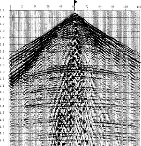
Figure 3 The shot record of Figure 1 after the application of a gain recovery algorithm to replace the energy lost as the signal traverses the earth. © Landmark/ITA.
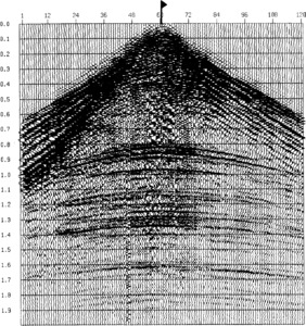
Figure 4 The shot record after a statistical deconvolution process has been applied to “shorten” the wavelet and increase time resolution. Copyright Landmark/ITA.
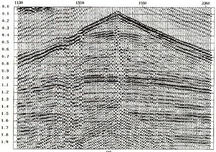
Figure 5a The application of statics corrects for differences in arrival time caused by elevation or weathering. (a) The valley in the data to the left of station 1500 represents an anomaly that persists throughout the time length of the record. Copyright Landmark/ITA.
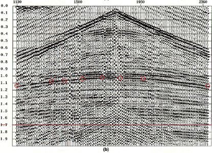
Figure 5b The application of statics corrects for differences in arrival time caused by elevation or weathering. (b) This “static” effect has been corrected. Copyright Landmark/ITA.

Given the broad categories of processing functions just described, this section briefly defines the common programs by their generic names in the order they would normally be applied. Some steps may be applied more than once at different times in the sequence, while others may be skipped for a particular dataset.

Demultiplex

The name given to sorting the traces from time ordered storage (all receiver stations at a given time) to receiver ordered format (all times for a given receiver) or trace sequential format. Many modern instruments do this in the field, but much data still comes in from the field multiplexed. SEG A and SEG B formats are multiplexed, SEG Y is a trace sequential format, and SEG D can be either way.

Edit

The process of flagging traces or pieces of traces to be ignored for one reason or another.

Geometry

The association by unique identifier of each recorded trace with shot and receiver locations.

Antialias filter

A low pass filter applied before resampling the data to a coarser time scale to prevent aliasing. Aliasing is a phenomenon in which high frequency data masquerades as low frequency energy as a result of undersampling. To sample a signal properly, there must be at least two samples within the shortest period of interest. Antialias filters remove frequencies above the sampling limit (Nyquist frequency) of the new sampling time. The operation is performed before the sampling is reduced.

Gain recovery

The correction for the loss in amplitude of a signal as it travels through the earth and spreads its energy over a larger surface area. This involves multiplication of the signal by a number that increases with time. The exact time variant multiplier can be based on the theoretical concept of spherical spreading (related to the square of the distance traveled), can be based on measurements of amplitude decay with time made on the data itself, or can be entirely arbitrary. An example of the effect of gain recovery is given in Figure 3.

Deconvolution

The removal of the frequency-dependent response of the source and the instrument. The instrument response is normally known and can be removed exactly. The source shape is not usually known but can be measured directly (marine air gun signatures) or estimated from the signal itself under certain assumptions. Signature deconvolution, wavelet deconvolution, spiking deconvolution, gapped deconvolution, predictive deconvolution, maximum entropy deconvolution, and surface consistent deconvolution are various manifestations of the attempt to remove the source width from the observed reflections.^[2] The resulting reflection sequence always has some smoothing function left, usually called the residual wavelet. Attempting to be too exact about deconvolution usually results in a very noisy section. The effect of deconvolution is seen in Figure 4.

Statics

The removal of traveltime artifacts relating to the placement of the source and receiver at or near the earth's surface. Differences in traveltime to the same reflector which result from elevation differences and near-surface velocity changes at different source and receiver stations must be removed. The relative elevation of each shot and receiver location and the near surface velocity must be known to make these corrections. An elevation datum is chosen, and the distance above or below that datum is measured for each source and receiver. The difficulty is in knowing what velocity to use to convert this elevation difference to a time correction to be added to or subtracted from the entire trace (hence the term statics). Refraction statics, surface consistent statics, and residual statics are all techniques used to estimate and apply the appropriate velocity and time corrections (Figure 5a and b).

Demultiple

Strong reflections can act as a secondary source of seismic energy that will interfere with the primary reflections and confuse the interpretation. Such secondary reflections are called multiples. The most common are water bottom multiples, but interbed multiples also exist. The demultiple process attempts to remove these^[2].

f–k or apparent velocity filter

Acoustic signals that are not reflections from subsurface layers appear in shot records (Figure 1) as straight lines rather than hyperbolic curves. These events have a constant “apparent velocity” as they travel along the receiver cable. This simple organization allows them to be isolated from the reflection signal and to be removed from the record. A common way to do this is with the FK (sometimes called pie slice) filter. Judicious selection of the range of apparent velocities to be removed can eliminate linear noise. Too wide a filter can remove too much information from the section and causes serious interpretation problems.

Normal moveout (NMO) correction

Figure 6 (a) A gather of processed traces with a common surface location. Shot-to-receiver offset is zero at the center of the gather and increases to about 2000 m deep on either end. The offset related curvature of the reflections is due to normal moveout. (b) Normal moveout correction (NMO) has been applied and the horizons are flat. The gather is now ready to be summed or stacked to produce one trace on Figure 2. Copyright Landmark/ITA.

The reflection from a given horizon does not arrive at the same time at different receivers along the length of the seismic cable or spread (see “Seismic Migration”). However, if the velocity at which the sound traveled is known, the arrival time difference (moveout) at each station can be predicted. Conversely, knowing the arrival time difference, the velocity the sound traveled can be determined under certain model assumptions. Usually the velocity of the earth as a function of time is determined at a few locations over the survey. This model can then be used to calculate moveout as a function of time everywhere in the survey. The moveout is subtracted from each seismic record such that the reflections from a given horizon will appear flat. This facilitates identification of reflectors and stacking. Figure 6 demonstrates the NMO process.

Dip moveout (DMO) correction

NMO corrections are made under the assumption of horizontal planar reflectors. If the reflector has appreciable dip, then the actual movement will be slightly different. The DMO correction is a method for estimating the effect of dip on moveout and removing it from the records as well.

Common midpoint (CMP) stack

This is the single most effective step for noise reduction in the processing flow. The shooting procedure results in many traces being acquired with the point midway between source and receiver (called the midpoint) being coincident on the earths surface. The only difference between the traces is the distance between source and receiver (offset). Once these traces have been NMO (and DMO) corrected, they are really redundant samples of the same reflection. Adding them together increases the signal to random noise ratio by the square root of the number of redundant samples. The process reduces the field data to a stacked section consisting of one trace for each midpoint location, assumed to have been recorded with a shot and receiver coincident at the midpoint location (see Figure 2).

Poststack filter

Usually a band pass filter, this process excludes frequencies above a certain value (high cut) and below a lower value (low cut) to retain that part of the signal with the highest signal to noise ratio. The values are usually set by trial and error and judged by a visual comparison of sections. The values may be different for different time gates of the section. Typically, the deeper reflections (later time) have less signal at high frequencies because these frequencies are absorbed or scattered more readily in the earth. Consequently, a lower value for the high cut frequency must be used as the bandpass is applied to later times on the trace.

Poststack mix

This is a simple procedure that averages together adjacent traces to enhance the signal to noise ratio. It causes a concurrent loss in horizontal resolution.

Migration, display and other advanced processing techniques are available and essential to the complete utilization of the seismic data.

Conclusions

Seismic processing attempts to enhance the signal to noise ratio of the seismic section and remove the artifacts in the signal that were caused by the seismic method. The end result should be a more interpretable section. The process has some very subjective elements. The selection of various parameters is done most often heuristically with more emphasis on satisfying the personal taste of the interpreter than on the rigorous physics of signal processing.

References

↑ ^1.0 ^1.1 Sheriff, R. E. 1984, Encyclopedic Dictionary of Exploration Geophysics: 2nd ed.: Tulsa, OK, Society of Exploration Geophysicists, 323 p.
↑ ^2.0 ^2.1 Yilmaz, O., 1987 Seismic Data Processing: Society of Exploration Geophysicists, Tulsa, OK, 525 p.

External links

find literature about
Seismic processing basics

[pt07r55-1] 1.0 ^1.1 Sheriff, R. E. 1984, Encyclopedic Dictionary of Exploration Geophysics: 2nd ed.: Tulsa, OK, Society of Exploration Geophysicists, 323 p.

[pt07r64-2] 2.0 ^2.1 Yilmaz, O., 1987 Seismic Data Processing: Society of Exploration Geophysicists, Tulsa, OK, 525 p.

[1]

[2]