Rock physics analysis for reservoir identification
| Wiki Write-Off Entry | |
|---|---|

| |
| Author | Radhi Muammar |
| Affiliation | Conrad Petroleum Ltd. |
| Competition | 2021 Middle East Wiki Write Off |

Rock physics addresses the relationship between the rocks’ elastic properties such as density, seismic wave velocities, and moduli as a function of composition, diagenetic processes, porosity, and fluid content. Such analysis is commonly carried out to discriminate between the reservoir and non-reservoir lithology, predict the reservoir’s expected seismic response, and to observe the relations of such elastic properties as a function of subsurface geology (rock physics diagnostic) by utilizing a given Vp-Vs-Rho set (P-wave, S-wave velocities, and density).
This article focuses on how this method can help solving such problems on a training dataset from clastic reservoir. The dataset is situated at a depth of 3,000-3,100 ft TVDSS in fluvial depositional environment. The lithology encountered in this interval comprised of two gas-charged sandstone bodies (clean and clayey sands) and claystones (mainly kaolinite).
Reservoir and Non-reservoir Lithology Discrimination[edit]
Reservoirs have distinctively different elastic properties compared to the non-reservoirs (shales, claystones, wet sands, etc.). An example from clastic gas reservoir is shown on Figure 1, where Sand A (clean sandstone) and Sand B (clayey sandstone as indicated by gamma ray log) have different density and wave velocities compared to the claystones, even Sand A and Sand B have different properties due to the presence of clays in Sand B.
In order to thoroughly discriminate the reservoir and non-reservoir lithology, the dataset should be derived into but not limited to the following properties:[1]
- AI (acoustic impedance) = this property is sensitive towards the change in lithology and fluid content. Gas has the lowest AI as it is acoustically softer compared to water, whereas oil sits in between. As this property is directly affected by the change in compaction and/or diagenetic processes, its sensitivity decreases under specific circumstances and may be unable to differentiate between each lithology.
- Vp/Vs (velocity ratio)= sensitive towards the change in fluid content even between wet and hydrocarbon bearing sandstones as Vp generally drops due to the presence of gas or oil however, the Vs does not affected much and therefore will produce low Vp/Vs. Velocity ratio is mathematically defined as follow:
- LR (lambda-rho)= good fluid indicator as it is sensitive to the change in fluid content. Lambda (Lamé parameter) is defined as fluid incompressibility, where gas has the lowest LR as it is highly compressible and least dense, water has the highest LR, whereas oil sits in between. LR is mathematically defined as follow:
- MR (mu-rho)= this property is sensitive towards the change in lithology. Sandstones generally have higher MR compared to shales and claystones due to its higher rigidity (μ). MR is mathematically defined as follow:
as MR is strongly controlled by the shear impedance (SI) and shear modulus (μ), the magnitude of this property does not really affected by pore fluids, but rather by the lithology.


As the available dataset is composed of gas saturated sands, one can model the expected elastic properties under wet condition by utilizing Gassmann’s Fluid Substitution.[2][3] The result of fluid substitution on Sand A and Sand B are shown on Figure 2. It can be observed that wet sands are acoustically harder (higher Vp and Rho, but with minor change in Vs) compared to gas sands, some of these wet sands are acoustically harder than the claystones.

These property differences can be easily highlighted on AI-Vp/Vs and LR-MR crossplots. On AI-Vp/Vs crossplot (Figure 3), it can be observed that claystones have higher AI and Vp/Vs compared with Sand A and Sand B (Sand A has the lowest AI and Vp/Vs). Some parts of Sand B have overlapping AI with claystone and therefore may exhibit uncertainties in discriminating the reservoir and non-reservoir lithology by utilizing this property. Vp/Vs on other hand, successfully separated the reservoir and non-reservoir lithology. In the case of wet sands, it can be observed that these sands have higher AI but smaller Vp/Vs. It can be concluded that AI may have some uncertainties to discriminate the reservoir and non-reservoir lithology (with the exception of clean gas sand), whereas Vp/Vs has a better performance result in separating them.

On LR-MR crossplot (Figure 4), it can be observed that claystones have the higher LR but lower MR compared to Sand A and Sand B, whereas Sand A has the lowest LR (attributed to the presence of gas that is easily compressible) but similar MR compared to Sand B as this property is more sensitive towards the change in lithology rather than fluid content. In the case of wet sands, the LR is similar to that of the claystones but with higher MR, similar to the gas sands.

These results suggest the validity of rock physics analysis to identify the presence of reservoir, where it successfully discriminate between Sand A, Sand B, wet sands and claystones. It should be noted that each property has their own functions and limitations. These crossplots can be utilized to determine the rock physics cut-off parameter for each lithology and later applied as a quality control for more advance geophysical methods such as seismic inversion.[1][4][5]
Predicting Reservoir’s Seismic Response[edit]
Seismic amplitude is defined by the difference of acoustic impedance between two layers, where higher difference in AI has “brighter” seismic amplitude at the interface between both layers such as the interface between claystone and high porosity gas sand that is indicated by sharp decrease in AI or the interface between claystone and tight carbonate that is indicated by sharp increase in AI. On well data, synthetic seismic (Figure 5) can be generated by convoluting reflectivity coefficient (product of the difference in AI between two layers) with a wavelet that is mathematically defined as follow:

where R is the reflectivity coefficient, AI1, Vp1, and Rho1 are the acoustic impedance, P-wave velocity, and density of the upper layer, whereas AI2, Vp2, and Rho2 are the acoustic impedance, P-wave velocity, and density of the lower layer. On Figure 5, (1) denotes the “bright” amplitude due to the sharp change in AI, whereas (2) denotes the “dim” amplitude due to the smaller change in AI.

To predict the seismic amplitude variation with offset (AVO) or angle (AVA), several approximations can be used.[6][7][8] To predict this AVO response however, Vs data is required. Figure 6 shows the expected seismic response between Sand A or Sand B (under gas saturated and wet condition) with their respective overlying and underlying claystones. It can be observed that under gas saturated condition, both sands have Class III AVO (increase in amplitude with increasing angle), whereas under wet condition, both sands have class II AVO (dim amplitude at Near and Far angle). It should be noted that different lithology (e.g. cemented sand and unconsolidated sand) may have different amplitude response. The occurrence of such sands can be interpreted by carrying out petrography analysis or rock physics diagnostic.
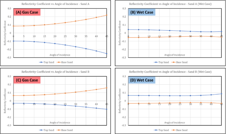
Figure 6 Expected AVO response of (A) Sand A under gas case, (B) Sand A under wet condition, (C) Sand B under gas case, and (D) Sand B under wet condition.
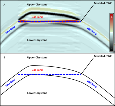
Figure 7 (A) Synthetic seismic of Sand A and (B) schematic cartoon of the modeled structure.


Synthetic seismic view of Sand A on an asymmetrical anticline structure is shown on Figure 7. Gas-water contact was modeled which properties were derived from fluid substitution. It can be observed that below the modeled GWC, amplitude polarity reversal can be identified due to the change from acoustically softer gas saturated sand to acoustically harder water saturated sand. This method is a common workflow to guide the seismic interpretation.
Rock Physics Diagnostic[edit]
This method was first introduced[9] to assess the change of velocity-porosity relations under different geological conditions, including pore shape, mineralogy, and post-depositional processes such as compaction and cementation (e.g. cemented sands are harder than uncemented rocks and compacted rocks at deeper depths are harder than the less compacted rocks at shallower depths due to the difference in effective stress).[10] Each of these geological conditions follows different velocity-porosity relations (rock physics model) and therefore, in absence of geological information (e.g. petrography), we can predict the cause of such velocity-porosity relations. Brief discussion these rock physics models are summarized below:[10]
- Friable Sand[9] = this rock physics model (unconsolidated line) shows the change in velocity-porosity relations as the sorting deteriorates. Well sorted sands are interpreted to have higher porosity and therefore, lower velocity. Grain deterioration decreases the porosity but only slightly stiffening the rock.
- Friable Shale[9] = similar rock physics model as above but the grain is modeled to be shale instead of sand.
- Contact Cement[11] = this rock physics model describes the change in velocity-porosity relations due to the cementation at grain contacts, effectively “gluing” the grains together. The cement at grain contacts significantly reinforcing the rock (large increase in velocity) but with small decrease of porosity.
- Constant Cement[12] = explains a sand body with varying sorting and porosity but with similar amount of cement in which the decrease of porosity is attributed to sorting deterioration. This model is an expansion of Friable Sand model that takes into account the impact of cement to the velocity-porosity relations.[10]
To conduct rock physics diagnostic, it is essential to eliminate as much variations as possible, such as saturation[9] because velocity depends on saturation. It is suggested to utilize the velocity log under wet condition to eliminate such variation. Figure 8 shows the total porosity-Vp crossplot of Sand A and Sand B where it can be observed that both sands follow the Friable Sand rock physics model indicating that the change in velocity and porosity of the sands are attributed to the difference in sorting.[9] Sand B has lower porosity but slightly higher velocity compared to Sand A due sorting deterioration caused by the clays.
As this approach may help interpreting the cause of such change in velocity-porosity relations as a function of subsurface geology in an area, this workflow can be utilized to predict the elastic properties of the rocks away from well control (e.g. to expect what seismic amplitude that corresponds to sand reservoir). Other examples of the application of this method have been reported by several authors.[13][14][15]

References[edit]
- ↑ 1.0 1.1 Goodway, B., T. Chen, and J. Downton, 1997, Improved AVO Fluid Detection and Lithology Discrimination using Lamé Petrophysical Parameters; “λρ”, “μρ”, and “λ/μ fluid stack”, from P and S Inversions: SEG Technical Program Expanded Abstracts, p. 183-186.
- ↑ Gassmann, F., 1951, Elastic Waves Through a Packing of Spheres: Geophysics, v. 16, no. 4, p. 673-685.
- ↑ Dvorkin, J., G. Mavko, and B. Gurevich, B., 2007, Fluid substitution in shaley sediment using effective porosity: Geophysics, v. 72, no. 3, p. O1-O8.
- ↑ Avseth, P., A. Janke, and F. Horn, 2016, AVO Inversion in Exploration – Key Learnings from a Norwegian Sea Prospect: The Leading Edge, v. 35, no. 5, p. 405-414.
- ↑ Sams, M., P. Begg, and T. Manapov, 2017, Seismic Inversion of a Carbonate Buildup: A Case Study: Interpretation, v. 5, no. 4, p. T641-T652.
- ↑ Aki, K. and P. G. Richards, 1980, Quantitative seismology: Theory and methods, San Francisco, W. H. Freeman and Co., 557 p.
- ↑ Shuey, R. T., 1985, A simplification of the Zoeppritz equations: Geophysics, v. 50, no. 4, p. 609-614.
- ↑ Fatti, J. L., G. C. Smith, P. J. Vail, P. J. Strauss, and P. R. Levitt, 1994, Detection of gas in sandstone reservoirs using AVO analysis: A 3-D seismic case history using the geostack technique: Geophysics, v. 59, no. 9, p. 1362-1376.
- ↑ 9.0 9.1 9.2 9.3 9.4 Dvorkin, J. and A. Nur, 1996, Elasticity of high-porosity sandstones: Theory for two North Sea data sets: Geophysics, v. 61, no. 5, p 1363-1370.
- ↑ 10.0 10.1 10.2 Avseth, P., T. Mukerji, G. Mavko, and J. Dvorkin, 2010, Rock-physics diagnostics of depositional texture, diagenetic alterations, and reservoir heterogeneity in high-porosity siliciclastic sediments and rocks–-A review of selected models and suggested work flows: Geophysics, v. 75, no. 5, p. 75A31-75A47.
- ↑ Dvorkin, J., A. Nur, and H. Yin, 1994, Effective properties of cemented granular material: Mechanics of Materials, v. 18, no. 4, p. 351-366.
- ↑ Avseth, P., J. Dvorkin, G. Mavko, and J. Rykkje, 2000, Rock physics diagnostic of North Sea sands: Link between microstructure and seismic properties: Geophysical Research Letters, v. 27, p. 2761-2764.
- ↑ Avseth, P., 2000, Combining rock physics and sedimentology for seismic reservoir characterization of North Sea turbiditsystems, Ph.D dissertation, Stanford University, Palo Alto, California.
- ↑ Hossain, Z. and L. MacGregor, 2014, Advanced rock-physics diagnostic analysis: A new method for cement quantification: The Leading Edge, v. 33, no. 3, p. 310-316.
- ↑ Antariksa, G., R. Muammar, and J. Lee, 2021, Performance evaluation of machine learning-based classification with rock-physics analysis of geological lithofacies in Tarakan Basin, Indonesia: Journal of Petroleum Science and Engineering, v. 208, part A, article 109250.