Difference between revisions of "Structurally complex reservoirs: evaluation"
Cwhitehurst (talk | contribs) m (added Category:Methods in Exploration 10 using HotCat) |
|||
| (48 intermediate revisions by 3 users not shown) | |||
| Line 11: | Line 11: | ||
| pdf = http://archives.datapages.com/data/specpubs/methodo1/images/a095/a0950001/0300/03310.pdf | | pdf = http://archives.datapages.com/data/specpubs/methodo1/images/a095/a0950001/0300/03310.pdf | ||
}} | }} | ||
| − | Evaluation of a structurally complex reservoir requires integration of geological and geophysical data to generate maps and cross | + | Evaluation of a structurally complex reservoir requires integration of geological and geophysical data to generate maps and [[cross section]]s that show the attitude, geometry, and thickness of key reservoir beds; the locations of crestal highs and [[Syncline|synclinal]] troughs; the position, [[dip]], and character of faults; and the location and orientation of the cutoffs of key beds on both sides of the faults. Also, fault blocks must be accurately delineated since they can effectively compartmentalize a reservoir. Maps and sections must be integrated so that they agree with each other, and they should be tested for viability and admissibility by balancing or [[backstripping]]. |
==Section construction== | ==Section construction== | ||
| + | <gallery mode=packed heights=300px widths=300px> | ||
| + | Evaluating-structurally-complex-reservoirs_fig1.png|'''Figure 1.''' SCAT plots used to define the complex structure seen in the discovery well of the Rail Road Gap oil field, California. The five plot types are (from left to right) [[azimuth]] versus depth (A plot), dip versus depth (D plot), dip versus depth in the direction of greatest curvature (T plot), dip versus depth in the direction of least curvature (L plot), and dip versus azimuth (DVA plot). (From Bengtsen.<ref name=Bengtson_1982 />) | ||
| + | Evaluating-structurally-complex-reservoirs_fig2.png|'''Figure 2.''' Predicted transverse and longitudinal cross sections and [[contour]] map derived from SCAT plots. Depths are subsea depths. (From Bengtsen.<ref name=Bengtson_1982 />) | ||
| + | Evaluating-structurally-complex-reservoirs_fig3.png|'''Figure 3.''' Cross section through an asymmetrical ramp anticline, Whitney Canyon field, Wyoming, with SCAT and isogen data superimposed. Uncomformities, axial planes, and inflection surfaces have been identified from the diameter data and projected away from the well bore. Isogens are contours of equal dip<ref name=Ramsay_1967></ref> and can constrain the shapes of [[fold]]s in section. (From Lammerson.<ref name=Lammerson1982>Lammerson, P. R., 1982, The Fossil basin and its relationship to the Absaroka thrust system, Wyoming & Utah, in R. B. Powers, ed., Geological Studies of the Cordilleran Thrust Belt: Rocky Mountain Association of Geologists, p. 279-340.</ref> | ||
| + | Evaluating-structurally-complex-reservoirs_fig4.png|'''Figure 4.''' Modeling extensional fault shapes from the rollover geometry. (a) the Groshong<ref name=Groshong_1989b>Groshong, R. H., 1989b, Structural style and balanced cross sections in extensional terranes: Houston Geological Society Short Course Notes, Feb. 24-25, 128 p.</ref> method uses oblique simple shear with a reference grid constructed with a spacing equal to the fault heave. Distance 2 from the rollover up to regional elevation of the same reference bed is transferred to 2′; likewise, 2′ + 4 is transferred to 4′ and so on to complete the fault trajectory. Interpolation between these points is carried out using a half grid spacing. (b) fault trajectory reconstruction by the Groshong<ref name=Groshong_1989b /> method uses simultaneous modeling of three horizons. Dashed trajectories are individual solutions; solid lines are the preferred solution. (From Hossack, unpublished data, 1988.) | ||
| + | Evaluating-structurally-complex-reservoirs_fig5.png|'''Figure 5.''' Example of a balanced section through a complex thrust ramp structure showing both the deformed and undeformed sections.<ref name=Mitra_1986>Mitra, S., 1986, [http://archives.datapages.com/data/bulletns/1986-87/data/pg/0070/0009/1050/1087.htm Duplex structures and imbricate thrust systems-Geometry, structural position, and hydrocarbon potential]: AAPG Bulletin, v. 70, p. 1087-1112.</ref> | ||
| + | </gallery> | ||
| + | |||
===Well and seismic constraints=== | ===Well and seismic constraints=== | ||
| − | Cross | + | [[Cross section]]s and maps are usually constructed simultaneously and need to be continually checked against each other (see [[Geological cross sections]] and [[Subsurface maps]]). The first well in a field provides depth, velocity, [[dipmeter]], and hydrocarbon distribution information that can improve the accuracy of predrill seismic and geological interpretations. Time pick corrections and seismic reprocessing generate improved seismic sections. Ideally, seismic sections should be time migrated and displayed with no vertical exaggeration so that true scale cross sections can be constructed for section restoration and balancing.<ref name=Dahlstrom_1970>Dahlstrom, C. D. A., 1970, Structural geology in the eastern margin of the Canadian Rocky Mountains: Canadian Society of Petroleum Geologists Bulletin, v. 18, p. 332-406.</ref> |
| − | Production wells may lie off the lines of seismic and geological section so that data will have to be projected carefully onto the lines using seismic cross lines or down-plunge projection.<ref name=DePaor_1988>DePaor, D., 1988, Balanced section in thrust belts, Part 1-- | + | Production wells may lie off the lines of seismic and geological section so that data will have to be projected carefully onto the lines using seismic cross lines or down-plunge projection.<ref name=DePaor_1988>DePaor, D., 1988, [http://archives.datapages.com/data/bulletns/1988-89/data/pg/0072/0001/0050/0073.htm Balanced section in thrust belts, Part 1--Construction]: AAPG Bulletin, v. 72, p. 73-90.</ref> |
===Orientation=== | ===Orientation=== | ||
| − | A balanced section can only be constructed in the direction of the regional displacement direction of the faults or in the direction of flexural slip on the fold limbs.<ref name=Dahlstrom_1970 /> The appropriate direction can be chosen by an analysis of regional structure maps using the bow string rule, lateral ramps, or drawing the section normal to the trend of the regional compressional or extensional folds.<ref name=Woodward_etal_1985>Woodward, N. B., S. E. Boyer, and J. Suppe, 1985, An outline of balanced cross sections, 2nd ed.: University of Tennessee Department of Geological Sciences, Studies in Geology 11.</ref> | + | A balanced section can only be constructed in the direction of the regional displacement direction of the faults or in the direction of flexural slip on the fold limbs.<ref name=Dahlstrom_1970 /> The appropriate direction can be chosen by an analysis of regional structure maps using the bow string rule, [[lateral]] ramps, or drawing the section normal to the trend of the regional compressional or extensional folds.<ref name=Woodward_etal_1985>Woodward, N. B., S. E. Boyer, and J. Suppe, 1985, An outline of balanced cross sections, 2nd ed.: University of Tennessee Department of Geological Sciences, Studies in Geology 11.</ref> |
===Structural style=== | ===Structural style=== | ||
Appropriate seismic lines, close to the line of section, define the structural style of the folds and faults, so this style should be incorporated directly into the section.<ref name=Dahlstrom_1970 /> Dip domain construction methods are popular guides to section drawing in both compressional and extensional systems.<ref name=Groshong_1989a>Groshong, R. H., 1989a, Half graben structures--balanced models of extensional fault bend folds: Geological Society of America Bulletin, v. 101, p. 96-105.</ref> | Appropriate seismic lines, close to the line of section, define the structural style of the folds and faults, so this style should be incorporated directly into the section.<ref name=Dahlstrom_1970 /> Dip domain construction methods are popular guides to section drawing in both compressional and extensional systems.<ref name=Groshong_1989a>Groshong, R. H., 1989a, Half graben structures--balanced models of extensional fault bend folds: Geological Society of America Bulletin, v. 101, p. 96-105.</ref> | ||
| − | |||
| − | |||
===Use of dipmeter=== | ===Use of dipmeter=== | ||
| − | Cross sections can be more highly constrained using statistical curvature analysis techniques (SCAT) on [[dipmeter]] data<ref name=Bengtson_1982>Bengtson, C. A., 1982, Structural and stratigraphic uses of dip profiles, in M. T Halbouty, ed., Deliberate Search for the Subtle Trap: AAPG Memoir 32, p. 31-45.</ref> ([[:Image: | + | Cross sections can be more highly constrained using statistical curvature analysis techniques (SCAT) on [[dipmeter]] data<ref name=Bengtson_1982>Bengtson, C. A., 1982, [http://archives.datapages.com/data/specpubs/basinar2/data/a130/a130/0001/0000/0031.htm Structural and stratigraphic uses of dip profiles], in M. T Halbouty, ed., Deliberate Search for the Subtle Trap: [http://store.aapg.org/detail.aspx?id=375 AAPG Memoir 32], p. 31-45.</ref> ([[:Image:Evaluating-structurally-complex-reservoirs_fig1.png|Figure 1]]). This method allows determination of the positions in a wellbore of important axial, crestal, and fault surfaces and their strike and dip ([[:Image:Evaluating-structurally-complex-reservoirs_fig2.png|Figure 2]]). Hence, structures can be projected in section away from wellbores and used to sketch the structure in profile. |
| − | |||
| − | |||
===Dip isogons=== | ===Dip isogons=== | ||
| − | |||
| − | [[ | + | ''Dip isogons,'' or [[contour]]s of equal dip in the plane of the section ([[:Image:Evaluating-structurally-complex-reservoirs_fig3.png|Figure 3]]),<ref name=Ramsay_1967>Ramsay, J. G., 1967, Folding and fracturing of rocks: New York and London, McGraw-Hill, 568 p.</ref> can be used to fill in the geological section. The isogons can be located from projected dipmeter data and projected or correlated between the wellbores following the rules described by Ramsay and Huber.<ref name=Ramsay_etal_1987>Ramsay, J. G., and M. I. Huber, 1987, The techniques of modern structural geology__Volume 2, in Folds and Fractures: Orlando, FL, Academic Press, 700 p.</ref> A series of dip segments along the various isogons helps the geologist sketch the fold profiles. Interpolation between the isogons can also be carried out using the dip domain methods previously described or by cubic spline interpolation.<ref name=McCoss_1987>McCoss, A. M., 1987, [http://www.sciencedirect.com/science/article/pii/0191814187900599 Practical section drawing through folded layers using sequentially rotated cubic interpolators]: Journal of Structural Geology, v. 9, p. 365-370.</ref> |
===Relationship of folding and faulting=== | ===Relationship of folding and faulting=== | ||
| − | Modern theories of structural geology generally relate the formation of folds to accommodation on irregular fault surfaces.<ref name=Hamblin_1965>Hamblin, W. K., 1965, Origin of "reverse drag" on the downthrown side of normal faults: Geological Society of America Bulletin, v. 76, p. 1145-1164.</ref> <ref name=Dahlstrom_1970 /> Generally, the folds are more obvious on seismic sections than faults, but fortunately there are geometric rules that allow us to predict one shape from the other<ref name=Suppe_1983>Suppe, J., 1983, Geometry and kinematics of fault-bend folding: American Journal of Science, v. 283, p. 684-721.</ref> <ref name=Verrall_1982>Verrall, P., 1982, Structural interpretation with applications to North Sea problems: Geological Society of London | + | Modern theories of structural geology generally relate the formation of folds to accommodation on irregular fault surfaces.<ref name=Hamblin_1965>Hamblin, W. K., 1965, [http://gsabulletin.gsapubs.org/content/76/10/1145 Origin of "reverse drag" on the downthrown side of normal faults]: Geological Society of America Bulletin, v. 76, p. 1145-1164.</ref> <ref name=Dahlstrom_1970 /> Generally, the folds are more obvious on seismic sections than faults, but fortunately there are geometric rules that allow us to predict one shape from the other<ref name=Suppe_1983>Suppe, J., 1983, [http://www.ajsonline.org/content/283/7/684.full.pdf+html Geometry and kinematics of fault-bend folding]: American Journal of Science, v. 283, p. 684-721.</ref> <ref name=Verrall_1982>Verrall, P., 1982, Structural interpretation with applications to North Sea problems: Geological Society of London Course Notes No 3, JAPEC (UK).</ref> <ref name=Gibbs_1983 />; Williams and Vann, 1987<ref name=Williams_etal_1987>Williams, G., and I. Vann, 1987, [http://www.sciencedirect.com/science/article/pii/0191814187900800 The geometry of listric normal faults and deformation in their hanging walls]: Journal of Structural Geology, v. 9, p. 789-795.</ref> <ref name=Groshong_1989a /> in both extensional and compressional examples. An example of a cross section solution explaining the relationship between extensional rollover and listric faults is shown in [[:Image:Evaluating-structurally-complex-reservoirs_fig4.png|Figure 4]]. |
| − | |||
| − | |||
===Balanced cross sections=== | ===Balanced cross sections=== | ||
| − | Balanced cross sections are used to test the viability or admissibility of a cross section. The deformed cross section is redrawn on a template in the undeformed state so that the beds are unfolded and the | + | Balanced cross sections are used to test the viability or admissibility of a cross section. The deformed cross section is redrawn on a template in the undeformed state so that the beds are unfolded and the [[offset]]s on the faults removed ([[:Image:Evaluating-structurally-complex-reservoirs_fig5.png|Figure 5]]). Section balancing requires reference pin-lines and loose lines at opposite ends of the section from which measurements of bed lengths are made. Bed thicknesses and bed lengths are generally retained so that the deformed and undeformed cross sections have the same area. For an ideal restoration, there should be no gaps or overlaps between adjacent fault blocks.<ref name=Woodward_etal_1985 /> |
| − | Balanced sections were first constructed for thrust belts, but Gibbs,<ref name=Gibbs_1983>Gibbs, A. D., 1983, Balanced cross section construction from seismic sections in areas of extensional tectonics: Journal of Structural Geology, v. 5, p. 153-160.</ref> Groshong,<ref name=Groshong_1989a /> and Rowan and Kligfield<ref name=Rowan_etal_1989>Rowan, M. G., and R. Kligfield, 1989, Cross section restoration and balancing as aid to | + | Balanced sections were first constructed for thrust belts, but Gibbs,<ref name=Gibbs_1983>Gibbs, A. D., 1983, [http://www.sciencedirect.com/science/article/pii/0191814183900408 Balanced cross section construction from seismic sections in areas of extensional tectonics]: Journal of Structural Geology, v. 5, p. 153-160.</ref> Groshong,<ref name=Groshong_1989a /> and Rowan and Kligfield<ref name=Rowan_etal_1989>Rowan, M. G., and R. Kligfield, 1989, [http://archives.datapages.com/data/bulletns/1988-89/data/pg/0073/0008/0950/0955.htm Cross section restoration and balancing as aid to seismic interpretation in extensional terranes]: AAPG Bulletin, v. 73, p. 955-966.</ref> have successfully applied the method to extensional and salt-related structures. Extensional section balancing is more difficult than compressional balancing because of the bed thickness changes that occur across faults. The balancing template has to show these thickness changes accurately. Generally, computer-aided methods are essential because they can sequentially backstrip the section to remove tectonic as well as compaction strains. Examples of these are described by Rowan and Kligfield,<ref name=Rowan_etal_1989 /> Worrall and Snelson,<ref name=Worrall_etal_1989>Worrall D. M., and S. Snelson, 1989, Evolution of the northern Gulf of Mexico with emphasis on Cenozoic growth faulting and the role of salt, in A. W. Bally and A. R. Palmer, The Geology of North America-An Overview: Geological Society of America, v. A, p. 97-138.</ref> and Shultz-Ela and Duncan.<ref>Schultz-Ela, D., and Duncan, K., 1990, Users manual and software for Restore, version 2.0: The Univ. of Texas Bureau of Economic Geology, 75 p.</ref> |
| − | + | ==Map construction== | |
| + | <gallery mode=packed heights=450px widths=450px> | ||
| + | Evaluating-structurally-complex-reservoirs_fig6.png|'''Figure 6.''' a) Structure map and b) restored structure map showing fault gaps removed. Remaining gaps and overlaps in the restored faults represent geometric incompatibilities in the interpretation. (From Galloway and Hobday.<ref name=Galloway and Hobday_1983>Galloway, W. E., and D. K. Hobday, 1983, Terrigenous clastic depositional systems applications to petroleum, coal, and uranium exploration: New York, Springer Verlag, 423 p.</ref>) | ||
| + | Evaluating-structurally-complex-reservoirs_fig7.png|'''Figure 7.''' Fault plane section and structure map of a model field to show the effects of Syncline|synclinal and cross fault spilling. (a) simple anticlinal closure cut by an extensional fault with two stacked reservoirs on both the downthrown and upthrown sides. Positions of cross fault spill points and synclinal spill points shown. (b) fault plane section illustrating the synclinal and cross fault spill points. Reservoir beds are shown hatchured, whereas seal horizons are shown white. Note the effect of thick seal trapping across the fault. (From Allan.<ref name=Allan_1989 />) | ||
| + | </gallery> | ||
| − | |||
===Structure contour maps=== | ===Structure contour maps=== | ||
| − | The geometry of the field is defined by a series of structure contour maps of key reservoir horizons ([[:Image: | + | The geometry of the field is defined by a series of structure [[contour]] maps of key reservoir horizons ([[:Image:Evaluating-structurally-complex-reservoirs_fig6.png|Figure 6a]]). The maps, showing several levels through the prospect or reservoir, are generated from well elevations of reference beds or depth-converted seismic sections (see [[Subsurface maps]]). Workstations for three-dimensional [[seismic interpretation]] considerably aid the process because the shapes of the structure contours and the faults are readily observable on horizontal seiscrop sections generated by the workstation.<ref name=Brown_1986>Brown, A. R., 1986, Interpretation of three-dimensional seismic data: [http://store.aapg.org/detail.aspx?id=1025 AAPG Memoir 42], 194 p.</ref> Contour maps can be quickly generated from stacked seiscrop sections. |
| − | |||
| − | |||
| − | |||
| − | |||
| − | + | Faults must be located in wellbores by omission (extension fault) or repetition (reverse fault) of stratigraphic section. These are defined on the electric logs by repetition or omission of parts of the SP and gamma ray signatures compared to a reference well that is believed to show an unfaulted section. Fault map trends and dip direction can also be defined by SCAT dipmeter analysis or on the stacked three-dimensional seiscrop sections. Generally, fault cuts have to be correlated from well to well to define the dip and curvature of the fault. Once these are estimated, fault contour maps can be generated by contouring the subsurface elevations of the fault cuts or, more directly, on the seismic workstation by stacking the seiscrop sections.<ref name=Brown_1986></ref> The faults will offset the reference beds, and the amount of offset in section and map view must be estimated. Once the separation is known, a separatin surface can be projected along the fault retaining the same trend, but adjusted in value by an amount appropriate for the offset on the fault (see [[:Image:Evaluating-structurally-complex-reservoirs_fig6.png|Figure 6a]]). | |
| − | Bed contours and fault contours have to be combined in a series of overlays to generate the structure map. Initially, individual fault blocks bounded on all sides by faults have to be contoured separately.<ref name=Dickinson_1954>Dickinson, G., 1954, Subsurface interpretation of intersecting faults and their effect upon stratigraphic horizons | + | Bed contours and fault contours have to be combined in a series of overlays to generate the structure map. Initially, individual fault blocks bounded on all sides by faults have to be contoured separately.<ref name=Dickinson_1954>Dickinson, G., 1954, [http://archives.datapages.com/data/bulletns/1953-56/data/pg/0038/0005/0850/0854.htm Subsurface interpretation of intersecting faults and their effect upon stratigraphic horizons]: AAPG Bulletin, v. 38, n. 5, p. 854-877.</ref> <ref name=Brown_1986></ref> The intersections between the bed and the fault contours of equivalent elevation value have to be identified to define the line of intersection of the bed and the fault. These lines are the fault cutoffs of the beds. There are two on each fault, one in the hanging wall and the other in the footwall. For extensional faults, there is a gap between the cutoffs where the key reference bed is omitted, and the gap in map view defines the heave across the fault. |
===Map restorations=== | ===Map restorations=== | ||
| − | Structure maps, like cross sections, can be tested for viability by restoring them to the undeformed state.<ref name=Barr_1985>Barr, D., 1985, 3D palinspastic restoration of normal faults in the Inner Moray Firth--implications for extensional basin development: Earth and Planetary Science Letters, v. 75, p. 191-203.</ref> Provided there are no areas of steep dip, a simple cut-and-paste restoration may highlight areas in the map where faults have been drawn inaccurately. [[:Image: | + | Structure maps, like cross sections, can be tested for viability by restoring them to the undeformed state.<ref name=Barr_1985>Barr, D., 1985, 3D palinspastic restoration of normal faults in the Inner Moray Firth--implications for extensional basin development: Earth and Planetary Science Letters, v. 75, p. 191-203.</ref> Provided there are no areas of steep dip, a simple cut-and-paste restoration may highlight areas in the map where faults have been drawn inaccurately. [[:Image:Evaluating-structurally-complex-reservoirs_fig6.png|Figure 6b]] shows a restoration where most of the individual fault blocks can be restored in map view to close up the fault gaps. The areas of overlap require additional redrafting or the collection of additional data. |
===Fault sealing characteristics=== | ===Fault sealing characteristics=== | ||
| − | The map patterns of oil-water and gas-oil contacts are important features that define field geometry. Common or separate oil-water contacts and gas-oil contacts in separate fault blocks will define sealing and nonsealing faults. The sealing characteristics of faults can also be gauged from the mud weights used during drilling or the production data from the well after completion. These data can be plotted on the maps and sections. A special type of section is the fault plane section of Allan | + | The map patterns of oil-water and gas-oil contacts are important features that define field geometry. Common or separate oil-water contacts and gas-oil contacts in separate fault blocks will define sealing and nonsealing faults. The sealing characteristics of faults can also be gauged from the mud weights used during drilling or the production data from the well after completion. These data can be plotted on the maps and sections. A special type of section is the fault plane section of Allan<ref name=Allan_1989>Allan, V. S., 1989, [http://archives.datapages.com/data/bulletns/1988-89/data/pg/0073/0007/0800/0803.htm Model for hydrocarbon migration and entrapment within faulted structures]: AAPG Bulletin, v. 73, p. 803-811,</ref> drawn within the plane of a single fault showing the positions of key reservoir and seal beds on either side of the fault and their contacts against one another across the fault ([[:Image:Evaluating-structurally-complex-reservoirs_fig7.png|Figure 7]]). This type of section allows the interpreter to perceive top seal and cross fault seal potential and pill points and to identify undrilled prospective fault blocks. Fault plane sections may have to be drawn in many different sections, particularly where faults cross-cut or splay off one another.<ref name=Allan_1989></ref><ref name=Downey_1984>Downey, M. W., 1984, [http://archives.datapages.com/data/bulletns/1984-85/data/pg/0068/0011/1750/1752.htm Evaluating seals for hydrocarbon accumulations]: AAPG Bulletin, v. 68, p. 1752-1763.</ref> <ref name=Smith_1966>Smith, D. A., 1966, [http://archives.datapages.com/data/bulletns/1965-67/data/pg/0050/0002/0350/0363.htm Theoretical considerations of sealing and nonsealing faults]: AAPG Bulletin, v. 50, p. 363-374.</ref> <ref name=Smith_1980>Smith, D. A., 1980, [http://archives.datapages.com/data/bulletns/1980-81/data/pg/0064/0002/0100/0145.htm Sealing and nonsealing faults in Louisiana Gulf Coast salt basin]: AAPG Bulletin, v. 64, p. 145-172.</ref> |
==See also== | ==See also== | ||
| Line 75: | Line 75: | ||
* [[Evaluating stratigraphically complex fields]] | * [[Evaluating stratigraphically complex fields]] | ||
* [[Evaluating diagenetically complex reservoirs]] | * [[Evaluating diagenetically complex reservoirs]] | ||
| + | {{clear}} | ||
==References== | ==References== | ||
| Line 85: | Line 86: | ||
[[Category:Geological methods]] [[Category:Test content]] | [[Category:Geological methods]] [[Category:Test content]] | ||
| + | [[Category:Methods in Exploration 10]] | ||
Latest revision as of 19:24, 19 January 2022
| Development Geology Reference Manual | |

| |
| Series | Methods in Exploration |
|---|---|
| Part | Geological methods |
| Chapter | Evaluating structurally complex reservoirs |
| Author | J. R. Hossack, D. B. McGuinness |
| Link | Web page |
| PDF file (requires access) | |
Evaluation of a structurally complex reservoir requires integration of geological and geophysical data to generate maps and cross sections that show the attitude, geometry, and thickness of key reservoir beds; the locations of crestal highs and synclinal troughs; the position, dip, and character of faults; and the location and orientation of the cutoffs of key beds on both sides of the faults. Also, fault blocks must be accurately delineated since they can effectively compartmentalize a reservoir. Maps and sections must be integrated so that they agree with each other, and they should be tested for viability and admissibility by balancing or backstripping.
Section construction[edit]
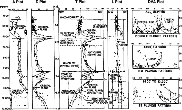
Figure 1. SCAT plots used to define the complex structure seen in the discovery well of the Rail Road Gap oil field, California. The five plot types are (from left to right) azimuth versus depth (A plot), dip versus depth (D plot), dip versus depth in the direction of greatest curvature (T plot), dip versus depth in the direction of least curvature (L plot), and dip versus azimuth (DVA plot). (From Bengtsen.[1])
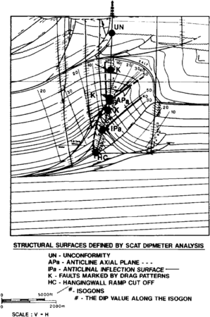
Figure 3. Cross section through an asymmetrical ramp anticline, Whitney Canyon field, Wyoming, with SCAT and isogen data superimposed. Uncomformities, axial planes, and inflection surfaces have been identified from the diameter data and projected away from the well bore. Isogens are contours of equal dip[2] and can constrain the shapes of folds in section. (From Lammerson.[3]
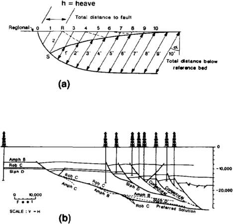
Figure 4. Modeling extensional fault shapes from the rollover geometry. (a) the Groshong[4] method uses oblique simple shear with a reference grid constructed with a spacing equal to the fault heave. Distance 2 from the rollover up to regional elevation of the same reference bed is transferred to 2′; likewise, 2′ + 4 is transferred to 4′ and so on to complete the fault trajectory. Interpolation between these points is carried out using a half grid spacing. (b) fault trajectory reconstruction by the Groshong[4] method uses simultaneous modeling of three horizons. Dashed trajectories are individual solutions; solid lines are the preferred solution. (From Hossack, unpublished data, 1988.)
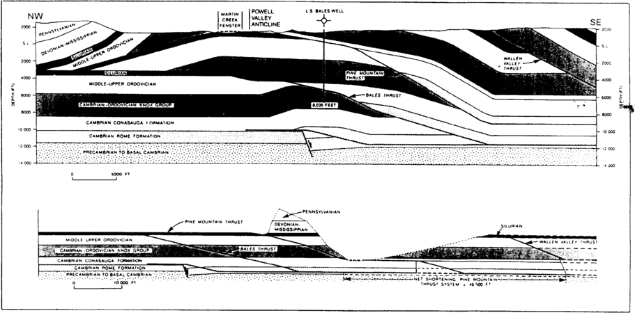
Figure 5. Example of a balanced section through a complex thrust ramp structure showing both the deformed and undeformed sections.[5]


Well and seismic constraints[edit]
Cross sections and maps are usually constructed simultaneously and need to be continually checked against each other (see Geological cross sections and Subsurface maps). The first well in a field provides depth, velocity, dipmeter, and hydrocarbon distribution information that can improve the accuracy of predrill seismic and geological interpretations. Time pick corrections and seismic reprocessing generate improved seismic sections. Ideally, seismic sections should be time migrated and displayed with no vertical exaggeration so that true scale cross sections can be constructed for section restoration and balancing.[6]
Production wells may lie off the lines of seismic and geological section so that data will have to be projected carefully onto the lines using seismic cross lines or down-plunge projection.[7]
Orientation[edit]
A balanced section can only be constructed in the direction of the regional displacement direction of the faults or in the direction of flexural slip on the fold limbs.[6] The appropriate direction can be chosen by an analysis of regional structure maps using the bow string rule, lateral ramps, or drawing the section normal to the trend of the regional compressional or extensional folds.[8]
Structural style[edit]
Appropriate seismic lines, close to the line of section, define the structural style of the folds and faults, so this style should be incorporated directly into the section.[6] Dip domain construction methods are popular guides to section drawing in both compressional and extensional systems.[9]
Use of dipmeter[edit]
Cross sections can be more highly constrained using statistical curvature analysis techniques (SCAT) on dipmeter data[1] (Figure 1). This method allows determination of the positions in a wellbore of important axial, crestal, and fault surfaces and their strike and dip (Figure 2). Hence, structures can be projected in section away from wellbores and used to sketch the structure in profile.
Dip isogons[edit]
Dip isogons, or contours of equal dip in the plane of the section (Figure 3),[2] can be used to fill in the geological section. The isogons can be located from projected dipmeter data and projected or correlated between the wellbores following the rules described by Ramsay and Huber.[10] A series of dip segments along the various isogons helps the geologist sketch the fold profiles. Interpolation between the isogons can also be carried out using the dip domain methods previously described or by cubic spline interpolation.[11]
Relationship of folding and faulting[edit]
Modern theories of structural geology generally relate the formation of folds to accommodation on irregular fault surfaces.[12] [6] Generally, the folds are more obvious on seismic sections than faults, but fortunately there are geometric rules that allow us to predict one shape from the other[13] [14] [15]; Williams and Vann, 1987[16] [9] in both extensional and compressional examples. An example of a cross section solution explaining the relationship between extensional rollover and listric faults is shown in Figure 4.
Balanced cross sections[edit]
Balanced cross sections are used to test the viability or admissibility of a cross section. The deformed cross section is redrawn on a template in the undeformed state so that the beds are unfolded and the offsets on the faults removed (Figure 5). Section balancing requires reference pin-lines and loose lines at opposite ends of the section from which measurements of bed lengths are made. Bed thicknesses and bed lengths are generally retained so that the deformed and undeformed cross sections have the same area. For an ideal restoration, there should be no gaps or overlaps between adjacent fault blocks.[8]
Balanced sections were first constructed for thrust belts, but Gibbs,[15] Groshong,[9] and Rowan and Kligfield[17] have successfully applied the method to extensional and salt-related structures. Extensional section balancing is more difficult than compressional balancing because of the bed thickness changes that occur across faults. The balancing template has to show these thickness changes accurately. Generally, computer-aided methods are essential because they can sequentially backstrip the section to remove tectonic as well as compaction strains. Examples of these are described by Rowan and Kligfield,[17] Worrall and Snelson,[18] and Shultz-Ela and Duncan.[19]
Map construction[edit]
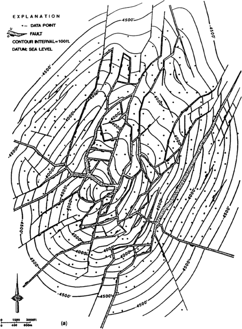
Figure 6. a) Structure map and b) restored structure map showing fault gaps removed. Remaining gaps and overlaps in the restored faults represent geometric incompatibilities in the interpretation. (From Galloway and Hobday.Cite error: Invalid
<ref>tag; invalid names, e.g. too many)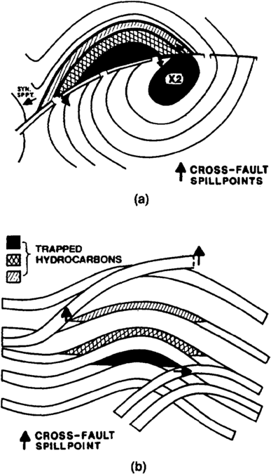
synclinal and cross fault spilling. (a) simple anticlinal closure cut by an extensional fault with two stacked reservoirs on both the downthrown and upthrown sides. Positions of cross fault spill points and synclinal spill points shown. (b) fault plane section illustrating the synclinal and cross fault spill points. Reservoir beds are shown hatchured, whereas seal horizons are shown white. Note the effect of thick seal trapping across the fault. (From Allan.[20])


Structure contour maps[edit]
The geometry of the field is defined by a series of structure contour maps of key reservoir horizons (Figure 6a). The maps, showing several levels through the prospect or reservoir, are generated from well elevations of reference beds or depth-converted seismic sections (see Subsurface maps). Workstations for three-dimensional seismic interpretation considerably aid the process because the shapes of the structure contours and the faults are readily observable on horizontal seiscrop sections generated by the workstation.[21] Contour maps can be quickly generated from stacked seiscrop sections.
Faults must be located in wellbores by omission (extension fault) or repetition (reverse fault) of stratigraphic section. These are defined on the electric logs by repetition or omission of parts of the SP and gamma ray signatures compared to a reference well that is believed to show an unfaulted section. Fault map trends and dip direction can also be defined by SCAT dipmeter analysis or on the stacked three-dimensional seiscrop sections. Generally, fault cuts have to be correlated from well to well to define the dip and curvature of the fault. Once these are estimated, fault contour maps can be generated by contouring the subsurface elevations of the fault cuts or, more directly, on the seismic workstation by stacking the seiscrop sections.[21] The faults will offset the reference beds, and the amount of offset in section and map view must be estimated. Once the separation is known, a separatin surface can be projected along the fault retaining the same trend, but adjusted in value by an amount appropriate for the offset on the fault (see Figure 6a).
Bed contours and fault contours have to be combined in a series of overlays to generate the structure map. Initially, individual fault blocks bounded on all sides by faults have to be contoured separately.[22] [21] The intersections between the bed and the fault contours of equivalent elevation value have to be identified to define the line of intersection of the bed and the fault. These lines are the fault cutoffs of the beds. There are two on each fault, one in the hanging wall and the other in the footwall. For extensional faults, there is a gap between the cutoffs where the key reference bed is omitted, and the gap in map view defines the heave across the fault.
Map restorations[edit]
Structure maps, like cross sections, can be tested for viability by restoring them to the undeformed state.[23] Provided there are no areas of steep dip, a simple cut-and-paste restoration may highlight areas in the map where faults have been drawn inaccurately. Figure 6b shows a restoration where most of the individual fault blocks can be restored in map view to close up the fault gaps. The areas of overlap require additional redrafting or the collection of additional data.
Fault sealing characteristics[edit]
The map patterns of oil-water and gas-oil contacts are important features that define field geometry. Common or separate oil-water contacts and gas-oil contacts in separate fault blocks will define sealing and nonsealing faults. The sealing characteristics of faults can also be gauged from the mud weights used during drilling or the production data from the well after completion. These data can be plotted on the maps and sections. A special type of section is the fault plane section of Allan[20] drawn within the plane of a single fault showing the positions of key reservoir and seal beds on either side of the fault and their contacts against one another across the fault (Figure 7). This type of section allows the interpreter to perceive top seal and cross fault seal potential and pill points and to identify undrilled prospective fault blocks. Fault plane sections may have to be drawn in many different sections, particularly where faults cross-cut or splay off one another.[20][24] [25] [26]
See also[edit]
- Introduction to geological methods
- Subsurface maps
- Geological cross sections
- Evaluating fractured reservoirs
- Evaluating stratigraphically complex fields
- Evaluating diagenetically complex reservoirs
References[edit]
- ↑ 1.0 1.1 1.2 Bengtson, C. A., 1982, Structural and stratigraphic uses of dip profiles, in M. T Halbouty, ed., Deliberate Search for the Subtle Trap: AAPG Memoir 32, p. 31-45.
- ↑ 2.0 2.1 Ramsay, J. G., 1967, Folding and fracturing of rocks: New York and London, McGraw-Hill, 568 p.
- ↑ Lammerson, P. R., 1982, The Fossil basin and its relationship to the Absaroka thrust system, Wyoming & Utah, in R. B. Powers, ed., Geological Studies of the Cordilleran Thrust Belt: Rocky Mountain Association of Geologists, p. 279-340.
- ↑ 4.0 4.1 Groshong, R. H., 1989b, Structural style and balanced cross sections in extensional terranes: Houston Geological Society Short Course Notes, Feb. 24-25, 128 p.
- ↑ Mitra, S., 1986, Duplex structures and imbricate thrust systems-Geometry, structural position, and hydrocarbon potential: AAPG Bulletin, v. 70, p. 1087-1112.
- ↑ 6.0 6.1 6.2 6.3 Dahlstrom, C. D. A., 1970, Structural geology in the eastern margin of the Canadian Rocky Mountains: Canadian Society of Petroleum Geologists Bulletin, v. 18, p. 332-406.
- ↑ DePaor, D., 1988, Balanced section in thrust belts, Part 1--Construction: AAPG Bulletin, v. 72, p. 73-90.
- ↑ 8.0 8.1 Woodward, N. B., S. E. Boyer, and J. Suppe, 1985, An outline of balanced cross sections, 2nd ed.: University of Tennessee Department of Geological Sciences, Studies in Geology 11.
- ↑ 9.0 9.1 9.2 Groshong, R. H., 1989a, Half graben structures--balanced models of extensional fault bend folds: Geological Society of America Bulletin, v. 101, p. 96-105.
- ↑ Ramsay, J. G., and M. I. Huber, 1987, The techniques of modern structural geology__Volume 2, in Folds and Fractures: Orlando, FL, Academic Press, 700 p.
- ↑ McCoss, A. M., 1987, Practical section drawing through folded layers using sequentially rotated cubic interpolators: Journal of Structural Geology, v. 9, p. 365-370.
- ↑ Hamblin, W. K., 1965, Origin of "reverse drag" on the downthrown side of normal faults: Geological Society of America Bulletin, v. 76, p. 1145-1164.
- ↑ Suppe, J., 1983, Geometry and kinematics of fault-bend folding: American Journal of Science, v. 283, p. 684-721.
- ↑ Verrall, P., 1982, Structural interpretation with applications to North Sea problems: Geological Society of London Course Notes No 3, JAPEC (UK).
- ↑ 15.0 15.1 Gibbs, A. D., 1983, Balanced cross section construction from seismic sections in areas of extensional tectonics: Journal of Structural Geology, v. 5, p. 153-160.
- ↑ Williams, G., and I. Vann, 1987, The geometry of listric normal faults and deformation in their hanging walls: Journal of Structural Geology, v. 9, p. 789-795.
- ↑ 17.0 17.1 Rowan, M. G., and R. Kligfield, 1989, Cross section restoration and balancing as aid to seismic interpretation in extensional terranes: AAPG Bulletin, v. 73, p. 955-966.
- ↑ Worrall D. M., and S. Snelson, 1989, Evolution of the northern Gulf of Mexico with emphasis on Cenozoic growth faulting and the role of salt, in A. W. Bally and A. R. Palmer, The Geology of North America-An Overview: Geological Society of America, v. A, p. 97-138.
- ↑ Schultz-Ela, D., and Duncan, K., 1990, Users manual and software for Restore, version 2.0: The Univ. of Texas Bureau of Economic Geology, 75 p.
- ↑ 20.0 20.1 20.2 Allan, V. S., 1989, Model for hydrocarbon migration and entrapment within faulted structures: AAPG Bulletin, v. 73, p. 803-811,
- ↑ 21.0 21.1 21.2 Brown, A. R., 1986, Interpretation of three-dimensional seismic data: AAPG Memoir 42, 194 p.
- ↑ Dickinson, G., 1954, Subsurface interpretation of intersecting faults and their effect upon stratigraphic horizons: AAPG Bulletin, v. 38, n. 5, p. 854-877.
- ↑ Barr, D., 1985, 3D palinspastic restoration of normal faults in the Inner Moray Firth--implications for extensional basin development: Earth and Planetary Science Letters, v. 75, p. 191-203.
- ↑ Downey, M. W., 1984, Evaluating seals for hydrocarbon accumulations: AAPG Bulletin, v. 68, p. 1752-1763.
- ↑ Smith, D. A., 1966, Theoretical considerations of sealing and nonsealing faults: AAPG Bulletin, v. 50, p. 363-374.
- ↑ Smith, D. A., 1980, Sealing and nonsealing faults in Louisiana Gulf Coast salt basin: AAPG Bulletin, v. 64, p. 145-172.
External links[edit]
| find literature about Structurally complex reservoirs: evaluation |