Shale-gas resource systems

Shale Reservoirs: Giant Resources for the 21st Century
Series	Memoirs
Chapter	Shale-gas Resource Systems
Author	Daniel M. Jarvie
Link	Web page
PDF	PDF file (requires access)
Store	AAPG Store

A shale resource system is described as a continuous organic-rich source rock(s) that may be both a source and a reservoir rock for the production of petroleum (oil and gas) or may charge and seal petroleum in juxtaposed, continuous organic-lean interval(s). As such, there may be both primary migration processes that are limited to movement within the source interval and secondary migration into nonsource horizons juxtaposed to the source rock(s). Certainly additional migration away from the resource system into nonjuxtaposed, noncontinuous reservoirs may also occur. In this scheme, fractured shale-oil systems, that is, shales with open fractures, are included as shale resource systems.

Two basic types of producible shale resource systems exist: gas- and oil-producing systems with overlap in the amount of gas versus oil. Although dry gas resource systems produce almost exclusively methane, wet gas systems produce some liquids and oil systems produce some gas. These are commonly described as either shale gas or shale oil, depending on which product predominates production. Although industry parlance commonly describes these as shale plays, these are truly mudstone; nonetheless, the term shale is used herein. It is important, however, to view these as a petroleum system, regardless of reservoir lithofacies or quality, because all the components and processes are applicable.

Given this definition of shale resource systems, these plays are not new with production from fractured mudstone reservoirs ongoing for more than 100 yr. Gas from Devonian shales in the Appalachian Basin and oil from fractured Monterey Shale, for example, have had ongoing long-term (100+ yr) production. The paradigm shift in the new millennium is the pursuit of tight mudstone systems, and although fractures may be present, they are usually healed with minerals such as calcite. Of course, having a brittle rock typically with a high silica content is also very important. These systems are organic-rich mudstones or calcareous mudstones that have retained gas or oil and have also expelled petroleum. The close association of source and nonsource intervals has sometimes made it difficult to ascertain which horizon is the actual source rock, for example, Austin Chalk and interbedded Eagle Ford Shale. Of course, in addition to retained or juxtaposed expelled petroleum, most of these organic-rich source rocks have expelled petroleum that has migrated, typically longer distances, into conventional reservoirs. The production success from shale-gas resource systems in North America has led to an international effort in exploration to identify such systems. This type of resource potential is present wherever a source rock is present, with risk ranging from and including geologic, geochemical, petrophysical, engineering, logistical, and economical to environmental factors. One clear advantage of shale-gas resource systems is the fact that they are the cleanest form of combustible carbon-based energy. Not only are particulate and smog-inducing components minimal, but also carbon dioxide emissions are the lowest for any carbon-based fuel.

An Appendix following Part 2 of this chapter provides maps with tabular legends referencing various worldwide shale resource plays, both gas and oil, that currently have wells drilled, in progress, or planned. Some speculative shale resource plays are included, and some prospective shale resource plays on this map will necessarily require updating based on drilling results. Certainly, other known source rocks are likely prospective as shale resource system plays, particularly marine shales, but also lacustrine and fluvial-deltaic systems.

Background

Producible natural gas shale resource systems in the United States provide a means of energy independence in natural gas for the foreseeable future. This may be for the next decade or for decades to come, depending on the economic, environmental, and political conditions for shale-gas production. This energy independence is created by the remarkable success achieved by the development of unconventional shale-gas resources. United States independent exploration and development companies have found and produced a huge surplus of natural gas, thereby making it a very inexpensive carbon-based energy source with a large remaining development potential.

Around the world, including Saudi Arabia, natural gas is being sought as a replacement for the far more valuable and expensive oil resource. The challenge is to develop and use this resource soundly, economically, safely, and effectively in our energy mix. It provides a means to an environmentally reasonable and abundant energy resource with a long production potential, thereby providing a bridge to the future until new energy sources are available at a reasonable cost and sufficient capacity to meet our industrial, social, and political needs—be they renewable or other forms of energy resources.

United States independent petroleum companies, led originally by Mitchell Energy and Development Corp. (MEDC), pursued and developed these unconventional shale-gas reservoir systems mostly during the last 10 yr in principal, although Mitchell's effort began much earlier. In 1982, drilling of the MEDC 1-Slay well Barnett Shale for its shale-gas resource potential was the launch point for this revolutionary exploration and production (EampP) effort. It was an incredibly difficult resource to exploit and was noncommercial through the 1980s and most of the 1990s. Even the first Barnett Shale horizontal well, drilled in 1991, the MEDC 1-Sims, was not an economic or even technical success. Horizontal drilling is an important part of the equation that has led to the development of shale resource plays, but it is only one component in a series of interlinked controls on obtaining gas flow from shale. For example, without understanding the importance of rock mechanical properties, stress fields, and stimulation processes, horizontal drilling alone would not have caused the shale-gas resource to develop so dramatically. Good gas flow rates in the 1990s were typically 1.4 times 104 m3/day (500 mcf/day) or less for most Barnett Shale wells, all of which were verticals except for the 1-Sims well. The economics were enhanced when MEDC began using slick-water stimulation to reduce costs, with the surprising benefit of improved performance in terms of gas flow rates. It was also learned that vertical wells could be restimulated, which raised production back to significant levels, commonly reaching or exceeding original gas flow rates. The use of technologies such as three-dimensional seismic and microseismic proved highly beneficial in moving the success of Barnett Shale forward. For example, a key point still argued to this day is the impact of structure and faulting on production potential. Obviously, conventional wisdom would suggest these as positive risk factors, when in fact they are typically negative. It was learned that stimulation energy was thieved by the presence of structures and faults, thereby typically lowering success when present. Application of microseismic surveys allowed engineers to map where the stimulation energy was being directed, thereby allowing adjustments to the stimulation program.

Ultimately, industry's use of horizontal wells and new technologies enhanced success in the Barnett Shale, and industry began to recognize its gas resource potential. However, the Barnett Shale-gas resource system was typically viewed as a unique case that could not be reproduced elsewhere.

The purchase of MEDC by Devon Energy in 2002 represented an industry paradigm shift. Devon's recognition of the potential of this resource led to their implementation of a very successful program for horizontal drilling. However, even with success and recognition of the Barnett Shale, companies were slow to recognize the broader potential of this type of resource system. Several events changed that perception: Devon's integration of a talented Devon Energy and MEDC Barnett Shale team, dramatically improved horizontal drilling results, Devonrsquos willingness to invest in new technologies to evaluate the play, the announcement by Southwestern Energy of success in the Fayetteville Shale in the Arkoma Basin of Arkansas, and the addition of, and movement from MEDC of, experienced, knowledgeable shale resource geologists and engineers to the general EampP pool. These factors led many companies to begin looking at shale resource potential.

The tenacity of George Mitchell, his compatriots at MEDC, and Devon and Southwestern Energy's successful drilling program in shale that led to the evolution of this play type cannot be overstated. Eventually, their successes brought the potential of shale-gas resource systems to national and, ultimately, global levels.

Characteristics of shale-gas resource systems

Figure 1 A simplified classification scheme for shale-gas resource systems. This typing schema uses gas type (biogenic versus thermogenic), source rock richness and thermal maturity, and lithofacies to categorize shale-gas systems into five basic continuous system types. The size of the circle is an indication of the resource potential.

Figure 2 Comparison of Montney Shale and Doig Phosphate in terms of total organic carbon (TOC) and porosity. The Montney Shale shows poor and inverse correlation to TOC, whereas the Doig Phosphate shows good and positive correlation indicative of organically derived porosity. The positive y-(porosity) intercept for the Doig indicates about 2% matrix porosity. The inverse correlation of the Montney Shale is suggestive of a hybrid system where porosity is derived primarily from matrix as opposed to organic porosity. BV = bulk volume; R2 = linear correlation coefficient.

What are the characteristics of these shale resource plays that caused them to be either overlooked or ignored? It was certainly not their source rock characteristics because most are organic-rich source rocks at varying levels of thermal maturity that have sourced conventional oil and gas fields in virtually every basin where they have been exploited. Although their petroleum source potential is well known, their rock properties were very unattractive for reservoir potential amplified by their recognition as not only source rocks, but also as seal or cap rocks, certifying their nonreservoir properties. However, their retention and storage capacity for petroleum was largely ignored and mud gas log responses noted with the somewhat derogatory shale-gas moniker. Because these shale resource plays were a combination of source rocks and seals, the retention of hydrocarbons is a factor that was overlooked. Diffusion, albeit a slow process, suggested that oil and especially gas were mostly lost from such rocks over geologic time. For example, modeling petroleum generation in the Barnett Shale indicates that maximum generation may have been reached 250 Ma. Because of a complex burial and uplift history, maximum generation could have been reached about 25 Ma, but nonetheless, retention of generated hydrocarbons to the present day was not perceived as likely or certainly not to a commercial extent. As such, even in a good seal rock, diffusion should have resulted in a substantial loss of gas, thereby limiting the resource potential of the system. The presence of fractures, although healed, and the presence of conventional oil and gas reservoirs in the Fort Worth Basin, suggested that expulsion and diffusion had possibly drained the shale. In addition, gas contents measured on the MEDC 1-Sims well, 1991, were not very encouraging, suggesting non-commercial amounts of gas.

Overlooked were various characteristics of organic-rich mudstones. They certainly have the capacity to generate and expel hydrocarbons, but they also have retentive capacity and a self-created storage capacity. Data from Sandvik et al. and Pepper suggest that expulsion is a function of both original organic richness and hydrogen indices as they relate to a sorptive capacity of organic matter. The work by Pepper suggests that only about 60% of Barnett Shale petroleum should have been expelled, assuming an original hydrogen index (HIo) of 434 mg HC/g TOC. By difference, this suggests that 40% of the generated petroleum was retained in the Barnett Shale, with retained oil ultimately being cracked to gas and a carbonaceous char, if sufficient thermal maturity (gt1.4% vitrinite reflectance equivalency [Roe]) was reached. This retained fraction of primary and secondarily generated and retained gas readily accounts for all the gas in the Fort Worth Basin Barnett Shale.

In addition, work by Reed and Loucks and Loucks et al. showed that the development of organic porosity was a feature of Barnett Shale organic matter at gas window thermal maturity. This was speculated to provide a means of storage by Jarvie et al. because of the conversion of organic matter to gas and oil, some of which was expelled, ultimately creating pores associated with organic matter. Conversion of TOC from mass to volume shows that such organic porosity can be accounted for by organic matter conversion. Likewise, it was shown that such limited porosity (4–7%) can store sufficient gas under pressure-volume-temperature (PVT) conditions to account for the high volumes of gas in place (GIP) in the Barnett Shale. In fact, it is postulated that PVT conditions during maximum petroleum generation 250 Ma were much higher than the present day, and despite uplift, the gas storage capacity is actually higher than present-day PVT conditions would suggest. If any liquids are present, however, condensation of petroleum occurs to accommodate the fixed volume under the lower temperature and pressure conditions after uplift. As such, a two-phase petroleum system exists, and this is an important consideration, not only for the Barnett Shale, but also for other resource systems containing both liquid and gas whereby liquids can condense on pressure drawdown.

Proof of the Barnett Shale-gas resource potential was substantiated by the MEDC 3-Kathy Keele well (now named the K. P. Lipscomb 3-GU) drilled in 1999, where pressure core was taken. The result was an estimate of 2.13 times 109 m3/km2 (195 bcf/section), which exceeded previous estimates by about 250%.

It should be noted that petroleum source rocks generate both oil and gas throughout the oil and early condensate-wet gas window. It is the relative proportion of oil to gas that describes the oil and gas windows; that is, oil is the predominant product in the oil window and gas in the gas window. Most of these plays are combination plays where both oil and gas are produced, the exception being dry gas window systems such as the Fayetteville Shale at 2.5% Ro. With the economic importance of liquid hydrocarbons, the pursuit of higher calorific gas with liquids or liquids with some gas has become the new paradigm.

Shale-gas resource systems evolved from the Barnett Shale work into a multitude of plays in North America that are now being pursued on a worldwide basis. Some commonalities among the systems exist, although many more differences are present. The best shale-gas resource system wells in core (best) producing areas in terms of initial production (IP) and ongoing production typically share these characteristics:

• Are marine shales commonly described as type II organic matter (HIo: 250–800 mg/g)
• Are organic-rich source rocks (gt1.00 wt. % present-day TOC [TOCpd])
• Are in the gas window (gt1.4% Roe)
• Have low oil saturations (lt5% So)
• Have significant silica content (gt30%) with some carbonate
• Have nonswelling clays
• Have less than 1000-ηd permeability
• Have less than 15% porosity, more typically about 4 to 7%
• Have GIP values more than 100 bcf/section
• Have 150+ ft (45+ m) of organic-rich mudstone
• Are slightly to highly over pressured
• Have very high first-year decline rates (gt60%)
• Have consistent or known principal stress fields
• Are drilled away from structures and faulting
• Are continuous mappable systems

Trying to classify shale-gas systems has proven to be an elusive task because of the high degree of variability among these systems and the range of descriptions from very simple to very detailed. A basic classification scheme includes a combination of gas type (biogenic versus thermogenic), organic richness, thermal maturity for thermogenic gas systems, and fracturing (whether open or closed) (Figure 1).

Hybrid systems are defined as those systems having a source rock combined with a higher abundance of organic-lean interbedded or juxtaposed nonclay lithofacies, for example, carbonates, silts, sands, or calcareous and argillaceous lime mudstones. As such, these hybrid resource systems have both source and nonsource intervals that allow access to gas in both lithofacies, although the nonsource lithofacies may be far more important because of its rock properties.

Although organic-rich mudstone systems commonly have a substantial organic porosity component, hybrid systems may have no organic porosity; they have predominantly matrix porosity or, in some cases, fracture porosity. The Triassic Doig Phosphate and Montney formations from the Western Canada sedimentary basin illustrate one such difference in organic richness and storage capacities in a mudstone versus a hybrid shale resource system. The Doig Phosphate is an organic-rich mudstone and has reasonably good correlation of bulk volume porosity to TOC, whereas the Montney Shale shows an inverse and poor correlation (Figure 2). In the case of the Doig Phosphate, this implies that organic porosity is the primary storage mechanism formed as a result of organic matter decomposition. However, the Montney Shale relies primarily on matrix porosity of petroleum expelled from organic-rich shales either within the Montney or from other sources. Other hybrid systems are a theme and variation of this; for example, the hybrid Eagle Ford Shale system is more aptly described as a calcareous or argillaceous lime mudstone with high TOC, and it has a high interbedded carbonate content (typically sim60%) that provides additional matrix storage capacity in intimately associated (juxtaposed) carbonates.

Organic richness: total organic carbon assessment

One of the first and basic screening analyses for any source rock is organic richness, as measured by total organic carbon (TOC). The TOC is a measure of organic carbon present in a sediment sample, but it is not a measure of its generation potential alone, as that requires an assessment of hydrogen content or organic maceral percentages from chemical or visual kerogen assessments. As TOC values vary throughout a source rock because of organofacies differences and thermal maturity, and even depending on sample type, there has been a lengthy debate on what actual TOC values are needed to have a commercial source rock. All organic matter preserved in sediments will decompose into petroleum with sufficient temperature exposure; for EampP companies, it is a matter of the producibility and commerciality of such generation. In addition, the expulsion and retention of generated petroleum must be considered. However, original quantity (TOC) as well as source rock quality (type) of the source rock must be considered in combination to assess its petroleum generation potential.

From a qualitative point of view, part of this issue includes the assessment of variations in quantitative TOC values that are altered by, for example, thermal maturity, sample collection technique, sample type (cuttings versus core chips), sample quality (e.g., fines only, cavings, contamination), and any high grading of core or cuttings samples. Documented variations in cuttings through the Fayetteville and Chattanooga shales illustrate variations due to sample type and quality as cuttings commonly have mixing effects. An overlying organic-lean sediment will dilute an organic-rich sample often for 10 to 40 ft (3 to 12 m). This is evident in some Fayetteville and Chattanooga wells with cuttings analysis, where the uppermost parts of the organic-rich shales have TOC values suggesting the shale to be organic lean. However, TOC values increase with deeper penetration into the organic-rich shale, to and through the base of the shale, but then also continuing into underlying organic-lean sediments, until finally decreasing to low values. This is a function of mixing of cuttings while drilling. The same issue in Barnett Shale wells was reported by MEDC, who also reported lower vitrinite reflectance values for cuttings than core (sim0.15% Ro lower). The big problem with this mixing effect is that it does not always occur and picking of cuttings does not typically solve the problem in shale-gas resource systems, although it may work in less mature systems. One solution is to minimize the quantitation of the uppermost sections (sim9 m [sim30 ft]) of a shale of interest when cuttings are used for analysis. The inverse of this situation is often identifiable in known organic-lean sediments below an organic-rich shale or coal. This latter effect is more obvious below coaly intervals, where TOC values will be high unless picked free of coal.

In any case, what is measured in any geochemical laboratory is strictly present-day TOC (TOCpd), which is dependent on all previously mentioned factors. In the absence of other factors, the decrease in original TOC (TOCo) is a function of thermal maturity due to the conversion of organic matter to petroleum and a carbonaceous char. The TOC measurements may include organic in oil or bitumen, which may not be completely removed during the typical decarbonation step before the LECO TOC analysis. Bitumen and oil-free TOC is described in various ways but always having two components whose distribution is dependent on the originally deposited and preserved biomass: generative organic carbon (GOC) and nongenerative organic carbon (NGOC) fractions. These have been referred to by various names without specifying bitumen and/or oil free (e.g., reactive and inert carbon). As such, the GOC fraction has sufficient hydrogen to generate hydrocarbons, whereas the NGOC fraction does not yield substantial amounts of hydrocarbons. Decomposition of the GOC also creates organic porosity, which is directly proportional to the GOC fraction and its extent of conversion. The NGOC fraction accounts for adsorbed gas storage and some organic porosity development due to restructuring of the organic matrix. The creation of such organic porosity in a reducing environment creates sites for possible catalytic activity by carbonaceous char or other catalytic materials, for example, low valence transition metals.

A slight increase in NGOC occurs as organic matter decomposes and uses the limited amounts of hydrogen in GOC (maximum of sim1.8 hydrogen to carbon [H-to-C] in the very best source rocks and about 2.0 H-to-C in bitumen and/or oil). Most shale-gas resource systems at a high thermal maturity have only small amounts or no GOC remaining and are dominated by the enhanced NGOC fraction. The decomposition of GOC generates all the petroleum, creates organic storage porosity, and both GOC and NGOC function in retention of generated petroleum that ultimately is cracked to gas in high-thermal-maturity shale-gas resource systems.

Original total organic carbon and hydrogen index determinations

• 

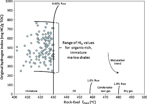
  Figure 3 Modified Espitalie et al. kerogen type and thermal maturity plot. A worldwide collection of immature marine shales shows a range of original hydrogen index (HI_o) values from approximately 250 to 800 mg HC/g TOC, with the majority plotting in the 300 to 700 mg HC/g TOC range. The key points are the range of values, and that all generate more oil than gas from primary cracking of kerogen. TOC = total organic carbon.

• 

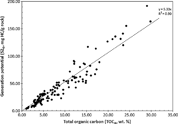
  Figure 4 Organofacies plot of original total organic carbon (TOCo) and original generation potential (S2o). These data show the high degree of correlation of the worldwide collection of marine shale source rocks. The slope of the correlation line is inferred to indicate the initial original hydrogen index (HI_o) value (533 mg HC/g TOC) for the entire group of source rocks with a y-intercept forced through the origin. R2 = linear correlation coefficient.

• 

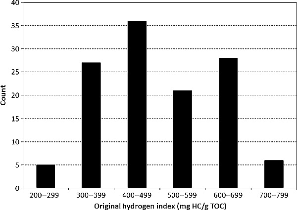
  Figure 5 Distribution of original hydrogen index (HI_o) values for a marine shale database containing immature samples. The highest percentage of HI_o values are in the 400 to 499 mg HC/g TOC range. Delimiting P90, P50, and P10 values from this distribution yields a P90 of 340, a P50 of 475, and a P10 of 645 mg HC/g TOC. TOC = total organic carbon.

Multiple ways to derive an original TOC (TOCo) value exist, two of which are (1) from a database or analysis of immature samples, thereby allowing the percentage of kerogen conversion to be estimated; and (2) by computation from visual kerogen assessments and related HI assumptions. However, it is difficult to assign an original HI (HI_o) to any source rock system in the absence of a collection of immature source rocks from various locations or even by measuring maceral percentages. For example, to assume all lacustrine shales such as the Green River Oil Shale have an HI_o of 700 or higher, or that all are equivalent to the Mahogany zone (950 mg HC/g TOC), is inconsistent with measured values that range from about 50 to 950 mg/g, with an average of only 534 mg HC/g TOC. Thus, our previous selection of 700 mg HC/g TOC for type I kerogen is likely overstated, and a comparable issue exists for organic matter categorized as a type II marine shale.

As most shale-gas resource plays to date have been marine shales, comparison of HI_o values for a worldwide collection of marine source rocks provides a means to assess the range of expected values. Using a database of immature marine source rocks, the predominant distribution of HI_o values is between 300 and 700 mg HC/g TOC, although the population of samples yield a range from about 250 to 800 mg HC/g TOC (Figure 3). This is similar to, but broader than, the range of values suggested by Peters and Caasa for type II kerogens of 300 to 600 mg HC/g TOC and slightly broader than the range of values suggested by Jones of 300 to 700 mg HC/g TOC. The important point is that these are primarily marine shales with oil-prone kerogen with variable hydrogen contents. Lacustrine source rocks are not ruled out as potential shale-gas resource systems, but they likely require a much higher thermal maturity to crack their dominantly paraffin composition to gas; as of this date, no such systems have been commercially produced.

Using these same data, an indication of this population average HI_o is given by the slope of a trend line established by a plot of TOCo versus the present-day generation potential (i.e., in this case, also original Rock-Eval measured kerogen yields [S2 or S2o]) (Figure 4). This graphic suggests an average HI_o of 533 mg HC/g TOC for this population of marine kerogens, assuming fit through the origin. However, using an average value is not entirely satisfactory either because these marine shales show considerable variation in HI_o, as shown by a distribution plot (Figure 5). Using this distribution, the likelihood of a given marine kerogen exceeding a certain HI_o value can be assessed, that is, application of P90, P50, and P10 factors. This distribution indicates that 90% of these marine shales exceed an HI_o of 340, 50% exceed 475, and only 10% exceed 645 mg HC/g TOC (Table 1):

Table 1. P90, P50, and P10 values for HI_o for a worldwide collection of marine source rocks.

	HIo (mg HC/g TOC)	GOC% of TOCo	NGOC% of TOCo
P90	340	55%	45%
P50	475	40%	60%
P10	645	29%	71%

^{HI_o = original hydrogen index; TOC = total organic carbon; GOC = generative organic carbon; NGOC = nongenerative organic carbon.}

If HI_o is known or taken as an average value or P50 value, the percent GOC in TOCo can readily be determined. Assuming that a source rock generates hydrocarbons that are approximately 85% carbon, the maximum HI_o can be estimated by its reciprocal, that is, 1/0.085 or 1177 mg HC/g TOC. The values for organic carbon content in hydrocarbons can certainly vary depending on the class of hydrocarbons and can range from about 82 to 88% (which would yield maximum HI_o values of 1220 and 1136 mg/g, respectively; the most commonly reported value in publications is 1200 mg HC/g TOC). However, from rock extract and oil fractionation data of marine shales or their sourced oils, the value of 85% appears sound with a plusmn3% variance.

Using 1177 mg HC/g TOC as the maximum HI_o, the percentage of GOC can be calculated from any HI_o, that is,

$\%{\text{ of reactive carbon}}={\text{HI}}_{\text{o}}/1177$

For example, if the HI_o of Barnett Shale is estimated to be 434 mg HC/g TOC, then dividing by 1177 mg/g yields the percentage of reactive carbon in the immature shale; that is, 37% of the TOCo could be converted to petroleum. As substantiation for this calculation, immature Barnett Shale outcrops from Lampasas County, Texas, average 36% reactive carbon, although the range of values is 29 to 43%. Similarly, data from Montgomery et al. suggest a 36% loss in TOCo on laboratory maturation of low-maturity Barnett Shale cuttings from Brown County, Texas. Likewise, immature Bakken Shale contains 60% GOC as carbon in Rock-Eval measured oil contents (S1) and measured kerogen yields (S2), which is consistent with an HI_o of 700 (59.5%).

This relationship for calculating the amount of GOC is true for any immature source rock once HI_o is determined or estimated. Using this relationship with HI_o probabilities, the range of original GOC and NGOC percentages for any HI_o can be determined. The values for GOC and NGOC for P90, P50, and P10 are also shown in Table 1. These values should not be considered mutually exclusive for a single source rock. Subdividing various organofacies within a source rock, if any, should be a common practice for calculating volumes of hydrocarbon generated with each organofacies having its own thickness, HI_o, and TOCo. Ideally, these organofacies differences should be mappable in an area of study.

• 

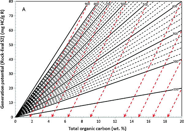
  Figure 6A (A-B) Iso-original hydrogen index (HI_o) (solid lines) and isodecomposition (dashed lines) on an original total organic carbon (TOCo) versus original S2 (S2o) nomograph. (A) Iso-HI_o lines from 100 to 900 mg HC/g TOC with isodecomposition lines illustrates the change in TOCo and S2o caused by kerogen conversion for the selected end point values.

• 

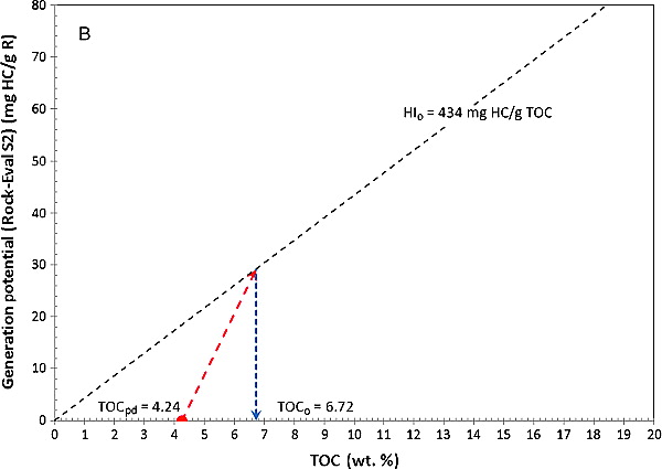
  Figure 6B (A-B) Iso-original hydrogen index (HI_o) (solid lines) and isodecomposition (dashed lines) on an original total organic carbon (TOCo) versus original S2 (S2o) nomograph. (B) Once the adjusted present-day TOC (TOCadj-pd) corrected for carbon in kerogen and bitumen and/or oil (see Table 2) is determined, the TOCo is derived by tracing the decomposition line to the HI_o intercept and dropping a perpendicular to the x-axis. S2 = Rock-Eval measured kerogen yields.

In lieu of these computations, a simple graphic can be used and is readily constructed in a spreadsheet. An HI_o isoline can be constructed for any HI_o using TOCo and S2o values. A nomograph is illustrated for every 20 mg/g of HI_o in the marine shale range of values in Figure 6A. Using the fact that the GOC is a function of HI_o/1177, the slopes for each 100 mg HC/g TOC value have isodecomposition lines that represent bitumen oil-free TOC and NGOC corrected for increased char formation by a simple function of 0.0004 times HI_o subtracted from base TOC values. Bitumen- and/or oil- and kerogen-free TOC is simply the subtraction of carbon in S1 and S2 from TOC, that is, {TOCpdminus (0.085 times (S1pd + S2pd))}. Regardless of HI_o or kerogen type, these isodecomposition lines are always parallel when 85% carbon in hydrocarbons is assumed.

Use of this nomograph is illustrated using data from the Barnett Shale (Figure 6B). Using a measured present-day TOC of 4.48%, with correction for bitumen and/or oil and kerogen in the rock and any increase in NGOC caused by hydrogen shortage, an original TOC of 6.27% is calculated. This means that the original generation potential (S2o) was 27.19 mg HC/g rock or, when converted to barrels of oil equivalent, 7.67 times 10minus2 m3/m3 (595 bbl/ac-ft). Data for this calculation are summarized in Table 2.

Table 2. Computation of original TOC from measured TOC and Rock-Eval data.

Geochemical Description	Value	Derivation
HIo	434	Estimated from all data
HIpd	28	$({\text{S2}}_{\text{pd}}/{\text{TOC}}_{\text{pd}}\times 100)$
TR	94%	$({\text{HI}}_{\text{o}}-{\text{HI}}_{\text{pd}})/{\text{HI}}_{\text{o}}$
TOCpd (wt. %)	4.48	Measured
S1pd (mg HC/g rock)	0.78	Measured
S2pd (mg HC/g rock)	1.27	Measured
%OC in S1+S2	0.17	$(0.085\times [{\text{S}}1_{\text{pd}}+{\text{S}}2_{\text{pd}}])$
TOCpdbkfree (wt. %)	4.31	$({\text{TOC}}_{\text{pd}}-{\text{OC in S}}1+{\text{S}}2)$
NGOCcorrection (wt. %)	0.35	$({\text{HI}}_{\text{o}}\times 0.0008)$
TOCpdNGOCadjusted (wt. %)	3.96	$({\text{TOC}}_{\text{pd, bkfree-NGOC correction}})$
%GOC in TOCo	37%	$({\text{HI}}_{\text{o}}/1177)$
TOCo (wt. %)	6.27	${\displaystyle ({\text{TOC}}_{\text{pd,}}{\text{ adjusted}}/(1-\%{\text{$GOC}})}
GOCo	2.31	wt. %
NGOCo	3.96	wt. %
S2o (mg HC/g rock)	27.19	${\displaystyle ({\text{$GOC}}_{\text{o}}/0.085)}
S2o (in boe/af)	595	boe/af $({\text{S}}2_{\text{o}}\times 21.89)$

^{TOC = total organic carbon; HI = hydrogen index; subscript ‘‘o’’ = original value; subscript ‘‘pd’’ = present-day measured or computed value; TR = transformation ratio, the change in original HI, where TR = (HI_o􏰂HIpd)/HI_o; GOC = generative organic carbon (in weight percentage); NGOC = nongenerative organic carbon (in weight percentage); bkfree = bitumen- and kerogen-free TOC values; subscript ‘‘NGOCcorrection’’ = minor correction to TOCpd for added carbonaceous char from bitumen and/or oil cracking. S1 = Rock-Eval measured oil contents; S2 = Rock-Eval measured kerogen yields; boe/af = bbl of oil equivalent per acre-ft.}

This nomograph provides a pragmatic method for estimating the elusive TOCo value and the original generation potential via determination of GOCo values when combined with either measured or estimated HI_o data or using a sensitivity analysis via P10, P50, and P90 HI_o values in the absence of other data. This is important because the total generation potential of the source rock can be estimated with these assumptions, and as such, the amount retained in the organic-rich shale can be estimated, that is, GIP, as well as the expelled amounts that may be recovered in a hybrid shale-gas resource system.

Where data are available showing variable organofacies in a given source rock interval, it is appropriate to subdivide the source rock by HI_o and TOCo. For example, if study of a source rock suggests multiple organofacies with different HI_o and TOCo values, the source rock should be subdivided into multiple units using the percentage of each to the total thickness of the source rock interval. For example, if 50% of a shale resource system is a leaner marine shale with an HI_o of 350 mg/g with a second organofacies constituting the other 50% of the shale and having an HI_o of 450 mg/g, then equation 1 becomes

$\%{\text{ of reactive carbon}}$

$=0.50\times (350/117)+0.50\times (450/1177)$

$=0.34{\text{or }}34\%{\text{ reactive organic carbon}}$

An important example of variable organofacies is provided by analog data for the Bossier and Haynesville shales in the area between the east Texas and north Louisiana salt basins. As only gas window maturity Bossier and Haynesville shale data are available, analog data are used, that is, immature Tithonian and Kimmeridgian source rocks from the deep-water Gulf of Mexico (Table 3).

Table 3. Averaged thickness and geochemical values on age-equivalent Bossier and Haynesville shale organofacies from deep-water Gulf of Mexico.

Organofacies	Percentage of Interval	Tmax °C	TOCo (wt. %)	HIo (mg HC/g TOC)	Generative Organic Carbon (% of TOCo)
Tithonian 3 (Bossier 3)	54	416	2.75	487	41
Tithonian 2 (Bossier 2)	24	436	1.02	299	25
Tithonian 1 (Bossier 1)	22	429	2.19	470	40
Kimmeridgian 2 (Haynesville 2)	60	411	5.60	720	61
Kimmeridgian 1 (Haynesville 1)	40	410	2.63	724	62

^{TOC_o = original total organic carbon; HI_o = original hydrogen index.}

The computed GOC values from these TOCo values are variable, ranging from about 25 (Bossier 2) to 62% (Haynesville 1). As previously suggested, such variation is good reason to segregate various organofacies of source rocks into percentages based on thickness instead of using a single average value. Differences in the Bossier and Haynesville shales have also been reported in the core-producing area of northwestern Louisiana on highly mature cuttings and core samples, although four facies were identified in the Bossier. A dramatic difference in the amount of GOC exists between the two formations and within the Tithonian itself. These organofacies differences in the Tithonian may explain the dramatic difference in TOC values reported for the Bossier Shale in Freestone County, Texas, and an unidentified location by Emme and Stancil. Available data for the Tithonian Bossier Shale suggest an about 1% TOC value on average in central Texas, with a value nearer 4% in easternmost Texas and in Louisiana.

Top 10 North American shale-gas plays

Table 4. Original hydrogen index, present-day TOC, original TOC, and P50-derived original TOC for top 10 shale-gas systems.

Formation	System or Series	HIo (mg/g)	TOCpd High (wt. %)	TOCpd Low (wt. %)	TOCpd Average (wt. %)	Standard Deviation (wt. %)	%GOC	%NGOC	TOCo Values			P50 (HI = 475)
									GOC (wt. %)	NGOC (wt. %)	TOCo (wt. %)	TOCo (wt. %)
Barnett	Mississippian	434	9.94	0.02	3.74	1.63	37	63	2.18	3.74	5.92	6.27
Fayetteville	Mississippian	404	7.13	0.71	3.77	1.74	34	66	1.97	3.77	5.74	6.32
Woodford	Devonian	503	11.27	0.26	5.34	2.28	43	57	3.99	5.34	9.33	8.95
Bossier	Upper Jurassic	419	4.11	0.46	1.64	1.06	36	64	0.91	1.64	2.55	2.75
Haynesville	Upper Jurassic	722	6.69	0.23	3.01	1.69	61	39	4.78	3.01	7.79	5.05
Marcellus	Devonian	507	9.58	0.41	4.67	3.05	43	57	3.53	4.67	8.20	7.83
Muskwa	Devonian	532	5.97	0.01	2.16	1.78	45	55	1.78	2.16	3.94	3.62
Montney	Triassic	354	4.78	0.01	1.95	0.67	30	70	0.84	1.95	2.79	3.27
Utica	Ordovician	379	3.06	0.19	1.33	0.72	32	68	0.63	1.33	1.96	2.23
Eagle Ford	Upper Cretaceous	411	5.6	0.58	2.76	1.11	35	65	1.48	2.76	4.24	4.63

Based on available data, HI_o values were derived or taken from immature sample populations for each of these source rocks (Table 4). These data show that most of these source rocks have HI_o values near P50 (475 mg/g), although the Haynesville Shale is higher than the P10 value. The values of TOCpd with minimum, maximum, and standard deviation and the TOCo from HI_o and P50 HI_o values for these top 10 shale-gas resource plays are also shown.

Figure 7 The TOCpd for the top 10 shale-gas resource systems. These data show the average TOCpd values for each system with the range of values, standard deviation, and number of samples. Given the high thermal maturity of these shales, these values are indicative of the nongenerative organic carbon (NGOC) values. TOCpd = present-day total organic carbon; stdev = standard deviation; n = number of samples.

The TOCpd values for shales of the shale-gas resource systems from various nonproprietary data sources are shown in Figure 7. These data or similar data are commonly cited in various company and financial industry reports. However, these numbers strictly represent TOCpd values and do not provide a good indication of the original hydrocarbon-generation potentials because they primarily represent NGOCpd, given that most are at gas window thermal maturity values. These TOCpd values do provide an indication of how much gas could be sorbed to the organic matter, however. If it is desired to show the true generation potential and make estimates of GIP, then TOCo and especially GOCo with derivation of original generation potential (S2o) are necessary.

Returning to the data in Figure 7, note that the TOCpd for the Barnett Shale is greater than the TOCpd for the Haynesville Shale. However, when corrected by HI_o for GOC, the Haynesville Shale has a higher hydrocarbon-generation potential. Interestingly, the GIP values reported for both the Barnett and Haynesville shales are comparable (e.g., sim150–200 bcf/section), and this is likely caused by the Haynesville Shale expelling more hydrocarbons (related to its higher HI_o value). As such, the higher gas flow rates in the Haynesville Shale are not a function of GIP, but instead a function of higher amounts of gas present because of higher porosity (and related higher free gas content) and higher pressure over a thinner shale interval than typically found in the Barnett Shale. Regardless, even if a P50 HI_o is used for the Haynesville Shale, it is likely that it has expelled a high percentage of the petroleum it generated based on the generation potential and related volumes of petroleum.

The available characteristics of these top 10 shale-gas resource systems are summarized in Table 5 for all available data or calculations.

Table 5. Available characteristics of the top 10 shale-gas resource systems in core-producing areas of each basin.

Shale	Marcellus	Haynesville	Bossier	Barnett	Fayetteville	Muskwa	Woodford	Eagle Ford	Utica	Montney
Basin or area	Appalachian Basin	East Texas-North Louisiana Salt Basin	East Texas-North Louisiana Salt Basin	Fort Worth Basin, Texas	Arkoma Basin, Arkansas	Horn River Basin, British Columbia	Arkoma Basin, Oklahoma	Eagle Ford-Austin Chalk trend, Texas	St. Lawrence Lowland, Quebec	Western Canada Sedimentary Basin, British Columbia, Alberta
Age	Devonian	Late Jurassic	Late Jurassic	Mississiappian	Mississiappian	Devonian	Devonian	Cretaceous	Ordovician	Triassic
Gas Type	Thermogenic	Thermogenic	Thermogenic	Thermogenic	Thermogenic	Thermogenic	Thermogenic	Thermogenic	Thermogenic	Thermogenic
Estimated Basin Area (mi2)	95,000	9000	9000	5000	9000	15,000	11,000	7500	2500	25,000
Typical Depth for Shale Gas (ft)	4000-8500	10,500-13,500	11,650	6500-8500	5700	7000-9000	6000-13,000	4000-10,000	2300-6000	3600-9000
Gross Thickness (ft)	190	225	280	200-1000	50-325	360-500	100-900	100-300	300-1000	900-1500
Net Thickness (ft)	50-350 (150)	200-300 (260)	200-300 (245)	100-700 (300)	20-200 (135)	400	100-220	150-300	500	350
Reported Gas Content (scf/ton)	60-150	100-330	50-150	300-350	60-220	90-110	200-300	200-220	70	300
Adsorbed Gas (%)	45	25	55	55	50-70	20	60	25	60	10
Free Gas (%)	55	75	45	45	30-50	80	40	75	40	90
Calorific Value (Btu)	1170	1050	1030	1050-1250	1040	1000	500-2000	1513	1350	1150
Porosity (%)	4.0-12.0 (6.2)	4.0-14.0 (8.3)	7.5	4.0-6.0 (5.0)	2-8 (6)	1-9 (4)	3-9 (5.0)	6-14		4-6
Permeability Range (Average) in nanodarcys	0-70 (20)	0-5000 (350)	0-100 (10)	0-100 (50)	0-100 (50)	0-200 (20)	0-700 (25)	700-3000 (1000)	0-50 (10)	5-75 (30)
Pressure Gradiant (psi/ft)	0.61	0.8	0.78	0.48	0.44	0.51	0.52	0.49	0.52	0.45
Gas-Field Porosity (%)	4	6	4	5	4.5	4	3	4.5	2.9	3.5
Water-Fill Porosity (%)	43	30	40-70	1.9	70	30	40	35	60	25
Oil Saturation (%)	1	<1	<1	10	<1	<1	5	15	5	1
Reported Silica Content (%)	37	30	25-30	45	35	60	55	15	12-51	40
Reported Clay Content (%)	35	30	35-50	25	38	20	20	15	15-26	15
Reported Carbonate Content (%)	25	20	5-25	15	12	10	5	60		30
Chlorite (%)	20 (0-50)	20 (0-50)	25 (10-50)	2.0 (0.0-20.0)	20 (5-40)	10 (0.0-30.0)	3 (0-40)	5 (0-50)	30 (5-50)	10 (0-40)
%Ro (average, range)	1.5 (0.9-5.0)	1.50 (1.20-2.40)	1.5 (1.10-2.40)	1.6 (0.85-2.1)	2.5 (2.0-4.5)	2.0 (1.4-2.2)	1.5 (0.7-4.0)	1.2 (0.8-1.6)	2.0 (0.8-3.0)	1.60 (0.90-2.50)
HI present-day	20	14	15	45	15	10	60	80	27	17
HI original	507	722	419	434	404	532	503	411	379	354
TR (%)	96	98	96	90	96	98	85	79	93	95
TOC present-day (average in wt. %)	4.01 (2.0-13.0)	3.01 (0.5-4.0)	1.64 (0.5-4.2)	3.74 (3.0-12.0)	3.77 (2.0-10.0)	2.16 (1.0-10.0)	5.34 (3.0-12.0)	2.76 (2.0-8.5)	1.33 (0.8-5.0)	1.95 (0.2-11.0)
TOC original (average in wt. %)	8.20	7.79	2.55	5.92	5.74	3.94	9.33	4.24	1.96	2.79
GOC original (average in wt. %)	3.53	4.78	0.91	2.18	1.97	1.78	3.99	1.48	0.63	0.84
S1 present day + S2 present day (mg/g)	1.23	0.71	0.40	1.95	0.35	0.62	4.05	3.76	2.25	0.67
S2 original (mg/g)	40.33	55.51	10.67	25. 65	23.18	20.95	46.91	17.42	7.43	9.87
Total Petroleum Yield (average in boe/af)	883	1215	234	519	500	445	938	299	113	201
Ethane Isotopic Rollover	Yes	Yes	Yes	Yes		Yes	Usually	Yes	Yes	Occasional
GIP from Gas Contents (average bcf/section)	130	190	165	150-200	55	150-260	40-120	40-223	25-160	10-110
Range of IPs (mcf/day)	3.0 (2.5-27.0)	8.4 (5.0-25.0)	5	1.5 (1.0-17.0)	1.3 (1.0-7.0)	5.0 (2.5-23.0)	1.9 (1.0-12.0)	5.0-17.0	1000	3.3 (1.5-6.0)
First year decline (%)	64	77	70 (est.)	64	65	71	66	70	65	54
Average EUR (horizontal) (bcfe)	3.7	5.8	3.5	1.7	1.3	4.8	2.2	5.5	1.4	3.4
Best (core) Production Area	Pennsylvania, West Virginia, New York	Northwestern Louisiana, east Texas	Northwestern Louisiana, east Texas	Wise and Johnson Counties, Texas	Eastern Arkoma	Northeast British Columbia	Western Arkoma, Oklahoma	Southeast Gulf Coast Texas	Quebec	British Columbia, Alberta

^{HI = hydrogen index; TR = transformation ratio; TOC = total organic carbon; GOC = generative organic carbon; GIP = gas in place; IP = initial production; EUR = estimated ultimate recovery; S1 = Rock-Eval measured oil contents; S2 = Rock-Eval measured kerogen yileds; boe/af = barrels of oil equivalent per acre-foot.}

Worldwide activity in shale-gas resource systems

Figure 8 Shale-gas risk plot showing various shales with their remaining present-day petroleum generation potential (S2pd) versus TOCpd. The area in red is the typical shale-gas productive values for HIpd (HIpdlt 100 mg/g), showing that these shales generally have shale-gas potentials ranging from very dry (HIpdlt 50 mg/g) to condensate-wet (HIpd 50–99 mg/g), indicating conversion of organic matter. HIpd values greater than 100 mg/g are indicative of oil window systems. TOCpd = present-day total organic carbon; HIpd = present-day hydrogen index; S2pd = present-day Rock-Eval measured kerogen yields.

Although shale-gas resource plays were slow to spread from the Barnett Shale into other United States and Canadian plays, a worldwide surge in interest has occurred since about 2006. The primary activity outside North America has been in Europe, where several companies including major oil and gas companies have secured land deals and have started drilling and testing of these plays. Key countries in this pursuit are Germany, Sweden, and Poland. The lower Saxony Basin of Germany has been studied extensively over the years. In the 1980s, the research organization KFA in Julich, Germany, was funded to drill shallow core holes into the lower Jurassic Posidonia Shale. In the Hils syncline area of the lower Saxony Basin, thermal maturity ranges from 0.49% to about 1.3% Ro. These cores and their published data provide a wealth of information on this Lower Jurassic source rock and potential resource play. The TOCo values average about 10.5%, with GOC values averaging 56% of the TOCo. Given the high oil saturations reported in the Posidonia Shale, there may be potential for shale-oil resource plays in the oil window parts of the basin.

Data for the Lower Cretaceous Wealden Shale is more difficult to locate, but some published TOC and Rock-Eval data on immature samples are available. These data suggest perhaps four different organofacies for the Wealden Shale, ranging in HIo from 500 to 700 mg HC/g TOC with variable TOCo contents ranging from about 4.5% to 8.0%. Generation potentials and TOC values for select samples from the Wealden and Posidonia shales are shown in Figure 8, with the highlighted red area being indicative of the core gas-producing area values for Barnett Shale in Fort Worth Basin, Texas. These data indicate that these shales are not highly converted, at least in this data set. Given this level of conversion, some liquids would be expected with gas, thereby having higher Btu values than other areas of the basin where maturities are higher. Certainly, once the areas of gas window thermal maturity are identified, it becomes necessary to assess other risk factors such as mineralogy, petrophysics, rock mechanics, and fluid sensitivities, for example.

ExxonMobil has now drilled at least four wells in the lower Saxony Basin for shale-gas resources, but no results are in the public domain.

In Sweden and Denmark, the Skegerrak-Kattegat Basin contains the Cambrian–Ordovician Alum Shale, which has also been studied extensively.. The Alum Shale is organic rich, with high TOC (11–22%) and HIo, yet generates primarily gas and condensate upon thermal conversion. Compositional yield data derived from immature Alum Shale with an HI of 487 mg HC/g TOC show that strictly primary kerogen and bitumen and/or oil cracking yields about 60% gas, quite unusual for source rocks of comparable HIo values that typically only yield 20 to 30% gas (D. M. Jarvie, unpublished data). Shell Oil Company has now drilled at least two wells into the Alum Shale, but no results are available.

Data from Poland suggest a variety of shale-gas potential in various basins such as the Baltic, Lublin, and Carpathian. Shale-gas resource potential exists in the Silurian Graptolitic Shale. Comparing data from across Poland using two criteria for shale-gas prospectivity, organic richness, and level of conversion, TOCpd values range from 2 to 18%, some with gas window levels of conversion (Figure 8). It is recently announced that the first shale stimulation in Europe has been completed on the 1-Markowolain well in the Lublin Basin. No gas flow data have been reported.

Other shale resource systems are being pursued in a variety of other basins in Europe as well. In Switzerland, the deep Vienna Basin will likely be tested for Posidonia Shale gas potential as will the Mikulov Shale in the Molasse Basin. Romania has also been under scrutiny for its shale-gas resource potential, but it may also have some shale-oil resource potential, given the good TOC values with low to modest conversion of organic matter (see Figure 8). Silurian–Devonian shales show good potential for shale-gas in Algeria and Tunisia (see Figure 8). In 2010, it was announced that the first stimulation of a potential shale-gas well was undertaken in the Ghadames Basin, west-central Tunisia, likely in the Silurian Tannezuft Shale.

In South Africa, the Karoo Basin is being evaluated for its shale-gas potential by various companies with various conventional and unconventional opportunities.

Saudi Aramco is also evaluating the potential for shale gas in the Kingdom of Saudi Arabia. Organic-rich and highly mature Silurian shales are being evaluated. This further illustrates the value of shale-gas resource systems as a more economical energy source than higher priced oil. The goal in Saudi Arabia would seem to be using shale-gas resources internally while exporting oil.

Several companies including BP, Shell, ConocoPhillips, Newfield, and EOG Resources have signed deals to explore for shale resource systems in China, covering five different basins. In the Sichuan Basin, Late Ordovician and Early Silurian marine shales are being evaluated for their shale resource potential. The Upper Ordovician Wufeng and Lower Silurian Longmaxi shales average about 3.0% TOC, with thermal maturities from about 2.3 to 3.4% Ro being targeted. In the Junggar Basin, the Jurassic Badaowan Shale has TOC values from 2 to 8%, with thermal maturities from 0.60 to 2.0% Roe and is 50 to 80 m (164–262 ft) thick. An excellent source potential also exists in the Upper Permian Lacaogou Formation (M. Burnaman, 2010, personal communication). The Triassic shales of the Ordos Basin and Jurassic shales of the Sichuan Basin are speculated to be shale-oil resource plays.

The Oil and Natural Gas Corp. of India (ONGC) is drilling its first shale resource system in the Damodar Basin, with an objective of a Permian shale with a thickness of about 700 m (sim2300 ft).

In Australia, Beach Energy has announced plans to test the Permian section of the Cooper Basin for shale gas. This is likely the Permian Roseneath Shale, which is highly mature in the basin (see Figure 8).

South America has shale resource activity in Argentina, Uruguay, Brazil, and Colombia, although most are for shale-oil resource systems. In Brazil's Parnaiba Basin, a shale-gas resource has been found in the Devonian Pimenteiras Shale. Of course, nearby the United States, activity has been high in Canada, whereas only recently has activity been under way in Mexico's Burgos Basin.

The worldwide exploration effort for shale-gas resource plays will continue for years to come and will likely impact global energy resources in a very positive way. Although recent concerns over groundwater contamination are of extreme importance to all of us both outside and within industry, it should be noted that more than 40,000 shale-gas wells have been hydraulically stimulated and more than one million conventional wells. Hype often takes precedence over facts as indicated, for example, by recent cases involving groundwater wells in the Fort Worth Basin. The United States Environmetal Protection Agency cited recent drilling operations in the Barnett Shale as the cause of these groundwater wells, but this was not substantiated. Geochemical data conclusively proved that although gas existed in these water wells, the gas migrated from shallow gas-bearing reservoirs in the basin and not from drilling operations in the Barnett Shale itself. Although there is and should be concern over any groundwater contamination issues, most of which are the result of ongoing geologic processes, the track record from drilling all the shale-gas wells and such evidence as cited in the Railroad Commission of Texas hearing provide support for the safe drilling record of industry. Accidents will occur in all industries, and human endeavors and regulations assist in minimizing such unwanted results by all parties, including companies doing the exploration and production, because their livelihoods also depend on positive impact. Perhaps the biggest concern should be the rapid expansion of shale-gas drilling that has stressed the need for availability of a qualified and knowledgeable workforce. As such, management and the supervision of work and drilling crews become perhaps of equal importance as regulatory efforts to improve environmental safety based on new geologic and chemical information.

Conclusions

The TOCpd values for high-thermal-maturity shales are typically only indicative of the nongenerative part of the TOC. The TOCo and its GOC content provide the key to hydrocarbon generation and organic storage (porosity) development. When HIo is known, %GOC can readily be determined by dividing the HIo by 1177. The TOCpd does provide an indication of adsorptive capacity of a shale.

Using a worldwide database of immature marine shales, it is determined that 90% of marine shales have an HI greater than 345, 50% greater than 475, and 10% greater than 640 mg HC/g TOC. An average value based on this database yields a value of 533 mg HC/g TOC for HIo.

A nomograph for predicting original TOC is provided. This graphic is based on determining HIo or using a P50 value for marine shales (475 mg HC/g TOC or the slope-derived value of 533 mg HC/g TOC). The P50 value for HIo shows a good comparison with most shale-gas resource systems and provides a basic means for assessing hydrocarbon-generation potentials. A sensitivity analysis is possible using P10, P50, and P90 values of HIo. However, when possible, measured values determined on immature rock samples should be used.

The success of shale resource systems in North America has provided impetus to identify these plays globally. Considerable effort is under way in Europe, China, and India to identify and test such resource systems. Even in oil-rich countries, interest exists in shale-gas resource systems as a cost-effective and environmentally friendly substitute for more expensive and valuable oil.

Shale-gas resource systems provide an ample source of carbon-based energy that can be used to mitigate the environmental impact, while powering worldwide consumption needs and reducing conflicts over the access to such energy. The result is a better world for us that bridges the gap to an environmentally neutral energy future.

gas in pipe

gas-oil contact

barrels

estimated ultimately recoverable

bridge plug