Three-dimensional modeling of clinoforms in shallow-marine reservoirs
| Three-dimensional modeling of clinoforms in shallow-marine reservoirs: Part 1. Concepts and application | |

| |
| Series | AAPG Bulletin, June 2015 |
|---|---|
| Author | Gavin H. Graham, Matthew D. Jackson, and Gary J. Hampson |
| Link | Web page |
Clinoform surfaces control aspects of facies architecture within shallow-marine parasequences and can also act as barriers or baffles to flow where they are lined by low-permeability lithologies, such as cements or mudstones. Current reservoir modeling techniques are not well suited to capturing clinoforms, particularly if they are numerous, below seismic resolution, and/or difficult to correlate between wells. At present, there are no modeling tools available to automate the generation of multiple three-dimensional clinoform surfaces using a small number of input parameters. Consequently, clinoforms are rarely incorporated in models of shallow-marine reservoirs, even when their potential impact on fluid flow is recognized.
A numerical algorithm that generates multiple clinoforms within a volume defined by two bounding surfaces, such as a delta-lobe deposit or shoreface parasequence, is developed. A geometric approach is taken to construct the shape of a clinoform, combining its height relative to the bounding surfaces with a mathematical function that describes clinoform geometry. The method is flexible, allowing the user to define the progradation direction and the parameters that control the geometry and distribution of individual clinoforms. The algorithm is validated via construction of surface-based three-dimensional reservoir models of (1) fluvial-dominated delta-lobe deposits exposed at the outcrop (Cretaceous Ferron Sandstone Member, Utah), and (2) a sparse subsurface data set from a deltaic reservoir (Jurassic Sognefjord Formation, Troll Field, Norwegian North Sea). Resulting flow simulation results demonstrate the value of including algorithm-generated clinoforms in reservoir models, because they may significantly impact hydrocarbon recovery when associated with areally extensive barriers to flow.
Introduction[edit]

Key factors influencing fluid flow and reservoir behavior include facies architecture and heterogeneity distribution conditioned to stratal surfaces. Within shallow-marine reservoirs, clinoforms are one such type of stratal surface. Clinoforms are dipping surfaces having geometry that preserves the depositional morphology of the delta-front or shoreface slope; and their distribution reflects the progradation history of the shoreline[2][3][4][5] (Figure 1). Clinoforms control aspects of detailed facies architecture within parasequences and can also act as low-permeability barriers or baffles to flow.[6][7][8][9][10][11][12] Therefore, it is important to include clinoforms in models of shallow-marine reservoirs to properly characterize facies architecture and volumes of hydrocarbons in place.[5] Under certain displacement conditions and if the clinoforms are associated with significant barriers to flow, clinoforms must be included in dynamic simulations to accurately predict likely drainage patterns and ultimate recovery of hydrocarbons.[11]
Standard modeling techniques are not well suited to capturing clinoforms, particularly if they are numerous, below seismic resolution, and/or difficult to correlate between wells. Few studies have attempted to identify and correlate clinoforms in the subsurface[13][14][15][16][17] or have built two-dimensional (2-D)[6][18] or three-dimensional (3-D)[9][10][11][5][12] flow simulation models that incorporate clinoforms. Previous studies of the Ferron Sandstone Member have incorporated simple clinoform geometries into reservoir models by using either object-based[10] or deterministic[9] approaches. Enge and Howell[12] used data collected by light detection and ranging (LIDAR) equipment to precisely recreate 3-D clinoform geometries from part of the Ferron Sandstone Member outcrops; the resulting flow-simulation model contained deterministically modeled clinoforms but in a volume smaller than most reservoirs (500 × 500 × 25 m [1640 × 1640 × 82 ft]). Sech et al.[5] used a surface-based modeling approach to produce a deterministic, 3-D model of a wave-dominated shoreface–shelf parasequence from a rich, high-resolution outcrop data set (Cretaceous Kenilworth Member, Utah), and Jackson et al.[11] used this model to investigate the impact of clinoforms on fluid flow. Jackson et al.[11] and Enge and Howell[12] both showed that capturing numerous clinoforms in fluid-flow simulations is feasible. Process-based forward numerical models are capable of generating geologically realistic, 3-D stratigraphic architectures containing clinoforms in shallow-marine strata (e.g., Edmonds and Slingerland;[19] Geleynse et al.[20]), but it can be difficult to replicate geometries observed in outcrop data, or condition models to subsurface data (e.g., Charvin et al.[21]); consequently, process-based approaches have yet to be developed for routine use in reservoir modeling.
Deterministic approaches are appropriate for modeling clinoforms that are tightly constrained by outcrop data, but they are time consuming to implement. Moreover, they do not allow flexibility in conditioning clinoform geometry and distribution to sparser data sets with a larger degree of uncertainty, such as those that are typically available for subsurface reservoirs. Incorporating hundreds of deterministic clinoform surfaces within a field-scale reservoir model would be a dauntingly time-consuming task, particularly if multiple scenarios and realizations that capture uncertainty in clinoform geometry and distribution are to be modeled. A stochastic, 3-D, surface-based modeling approach is required to address these issues. Similar approaches have been demonstrated for other depositional environments (e.g., Xie et al.;[22] Pyrcz et al.;[23] Zhang et al.[24]) and to create models of generic, dipping barriers to flow (e.g., Jackson and Muggeridge[25]), but at present, there are no tools available to automate the generation of multiple 3-D clinoforms using a small number of parameters. The aims of this paper are to develop an efficient, quick, and practical method for incorporating clinoforms into models of shallow-marine reservoirs and to validate its application through building both geologic and fluid-flow simulation models.
The paper is structured in four parts. First, we present a simple conceptual framework to describe clinoform geometries and distributions, which allows them to be incorporated into reservoir volumes deposited in different shallow-marine environments. The framework is used to develop an algorithm-based method to represent clinoform surfaces, which is sufficiently flexible to match clinoform geometries and distributions observed in rich outcrop data sets and also to honor sparse subsurface data. The second part of the paper validates the clinoform-modeling algorithm via construction of a 3-D reservoir model of a single fluvial–deltaic parasequence using high-resolution outcrop data from fluvial-dominated delta-lobe deposits in the Cretaceous Ferron Sandstone Member of east-central Utah. The model is constructed using a framework of surfaces, including flooding surfaces between parasequences, surfaces that represent clinoforms, and surfaces that represent boundaries between facies associations. The third part of the paper demonstrates an application of the clinoform-modeling algorithm to generate a reservoir model using a sparse subsurface data set from the deltaic Jurassic Sognefjord Formation, in a fault-bounded sector of the Troll Field, offshore Norway. The clinoform-modeling algorithm allows flexibility in building a range of surface-based reservoir models that incorporate uncertainty in heterogeneities associated with clinoforms. The resulting 3-D surface-based reservoir models are suitable for flow simulation without upscaling. Finally, in the fourth part of the paper, we demonstrate that the algorithm produces models suitable for flow simulation using the Ferron Sandstone Member outcrop analog and subsurface Sognefjord Formation examples. This latter step is missing in many papers that report new reservoir modeling algorithms. The simulation models are used to assess the potential impact of flow barriers associated with clinoforms on drainage patterns and hydrocarbon recovery.
The impact of clinoforms on flow and hydrocarbon recovery in the context of other uncertain reservoir geologic parameters and reservoir engineering decisions remains poorly understood. In a companion article, Graham et al.[26] apply the clinoform-modeling algorithm to build a reservoir-scale model of the Ferron Sandstone Member that incorporates multiple, stacked parasequences and provides a case study for fluvial-dominated deltaic reservoirs. The impact of clinoforms on fluid flow in the context of other uncertain reservoir geologic parameters, such as the presence of distributary and fluvial channels, the magnitude of permeability contrasts between facies associations, and the impact of bed-scale heterogeneity on vertical permeability, as well as reservoir engineering decisions including production rates are investigated.
Conceptual framework for clinoform modeling[edit]

Clinoforms occur at a wide range of spatial scales, from large, basinward-dipping surfaces at the shelf-slope margin, to smaller surfaces associated with progradation of deltaic and shoreface systems across the shelf (e.g., Helland-Hansen and Hampson[27]). This study focuses on developing a surface-based approach to represent clinoforms at any lengthscale in reservoir models, with emphasis on clinoforms produced by the progradation of deltaic, barrier-island, and strandplain shorelines, which are typically up to a few tens of meters in height. The 3-D geometry and spatial arrangement of shoreline-scale clinoforms reflect in large part the process regime under which they were deposited (e.g., Galloway[28]). Fluvial-dominated deltas exhibit a hierarchy of point-sourced, teardrop-shaped sediment bodies that are fed via a downstream branching network of distributary channels. From small to large lengthscales, this hierarchy consists of mouth bars, mouth-bar assemblages, and delta lobes[29] (equivalent to the jet-plume deposits, jet-plume-complex deposits, and delta lobes of Wellner et al.[30]). Sediment-body geometry is modified by the action of waves and tides, which respectively tend to result in shoreline-parallel and shoreline-perpendicular sediment transport that suppresses branching and switching of distributary channels (e.g., Galloway;[28] Willis;[31] Bhattacharya;[29] Plink-Björklund[32]). Clinoforms exist as a preserved record of sediment-body morphologies at each of these hierarchical lengthscales (e.g., Gani and Bhattacharya[33]) but are most commonly described at the scale of delta lobes in outcrop and high-resolution, shallow seismic data. For example, in Pleistocene fluvial-dominated delta deposits imaged in shallow-seismic data, Roberts et al.[34] comment that “each clinoform set represents rather continuous deposition from a distributary or related set of distributaries, resulting in the formation of a delta lobe.” Shale drapes and cemented concretionary layers occur along depositional surfaces at each hierarchical level but generally have greater continuity and extent at larger lengthscales of the hierarchy (e.g., Gani and Bhattacharya;[33] Lee et al.;[35] Ahmed et al.[36]). Thus, delta lobes tend to be overlain across flooding surfaces by prodelta shales and distal-delta-front heteroliths, which may cause them to behave as distinct reservoir zones that can be correlated between wells, whereas clinoforms are associated with heterogeneity between wells and within reservoir zones (e.g., Ainsworth et al.,;[7] Hampson et al.[17]).
The clinoform-modeling algorithm developed here is simple to use, requiring specification of only a few input parameters: (1) the upper and lower surfaces that define the rock volume within which the clinoforms are to be modeled; (2) the plan-view geometry of clinoforms; (3) clinoform geometry in depositional-dip-oriented cross section; and (4) spacing and progradation direction of the clinoforms. The user can also use a stochastic component of the clinoform-modeling algorithm if there are uncertainties in the parameter values to be used.
Bounding Surfaces That Define Rock Volume[edit]
Each set of shoreline clinoforms is contained within a distinct, upward-shallowing, regressive succession, or parasequence (sensu Van Wagoner et al.;[37] Hampson et al.,[17]), that is bounded at its base and top by flooding surfaces. Multiple clinoforms exist within each parasequence. Because the algorithm is generic, any top and base bounding surfaces can be used; the only requirement is that the top bounding surface is entirely above, or coincident with, the base bounding surface across the model volume (Figure 1A–C). By using the flooding surfaces at the top and/or base of a parasequence as reference surfaces, the algorithm can produce clinoforms that are modified by postdepositional folding and faulting (Figure 2A), truncation by overlying erosion surfaces (Figure 2B), and/or progradation over irregular sea-floor topography (Figure 2C). The parasequence-bounding flooding surfaces are first read into the clinoform-modeling algorithm, using a standard gridded format exported from a reservoir modeling software package. Clinoforms created by the algorithm adapt to the morphology of either (or both) bounding surfaces, using a height function, h(rc) (Figure 2D), that calculates the height of the clinoform relative to the length along the clinoform surface and the height difference between the top and base bounding surfaces (see Table 1 for nomenclature):
![{\displaystyle h(r_{c})=(h_{\text{max}}(r_{c})-h_{\text{min}}(r_{c}))-\left[{\frac {(r_{c}(x,y)-r_{\text{min}}(x,y))}{(r_{\text{max}}(x,y)-r_{\text{min}}(x,y)}}(h_{\text{max}}(r_{c})-h_{\text{min}}(r_{c}))\right]}](https://wikimedia.org/api/rest_v1/media/math/render/svg/6b0893d4a1504f541d7cdbdb668e37313a25815f)
| Parameter | Description | Units | Stochastic Modeling Component |
|---|---|---|---|
| bD | Length of base ellipse in depositional dip direction | m | ✓ |
| bS | Length of base ellipse in depositional strike direction | m | ✓ |
| c(rc) | Clinoform shape function | m | N/A |
| h(rc) | Height function, to give height of clinoform at rc(x, y) | m | N/A |
| hmax(rc) | Maximum height of top bounding surface at rc(x, y) | m | N/A |
| hmin(rc) | Minimum height of top bounding surface at rc(x, y) | m | N/A |
| L | Clinoform length | m | ✓ |
| P | Shape function exponent | None | ✓ |
| pO | Axis of progradation relative to bounding surfaces | None | ✓ |
| rc(x, y) | Radius from clinoform origin to point on surface | m | N/A |
| rmax(x, y) | Radius of base ellipse relative to clinoform origin | m | N/A |
| rmin(x, y) | Radius of top ellipse relative to clinoform origin | m | N/A |
| S | Clinoform spacing | m | ✓ |
| s(rc) | Shape function (power law for concave-upward geometry) | None | N/A |
| θ | Clinoform progradation angle relative to north | ° | ✓ |
| tD | Length of top ellipse in depositional dip direction | m | ✓ |
| tS | Length of top ellipse in depositional strike direction | m | ✓ |
| x | x coordinate on surface | None | N/A |
| xorigin | x coordinate of clinoform origin on surface | None | N/A |
| y | y coordinate on surface | None | N/A |
| yorigin | y coordinate of clinoform origin on surface | None | N/A |
*N/A = not applicable.
This allows the clinoforms to adapt to the morphology of the bounding surfaces (Figure 2A). For cases in which an overlying erosional bounding surface is interpreted to truncate clinoforms (Figure 2B) and/or clinoforms are interpreted to downlap onto a bounding surface that reflects irregular sea-floor topography (Figure 2C), a planar and horizontal dummy surface is used either above the erosional bounding surface or below the bounding surface, reflecting irregular sea-floor topography. The height function h(rc) (equation 1), is applied to the planar dummy surfaces to insert clinoforms; and, in a final step, the bounding surface geometries are used to remove the upper and/or lower portions of the clinoforms, where appropriate, to match interpreted truncation (Figure 2B) and/or down lap (Figure 2C).
Plan-View Clinoform Geometry[edit]
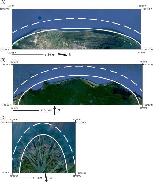
Figure 3 Generalized, first-order approximations of the plan-view geometry of clinoforms in different depositional environments: (A) Nayarit Coast, Mexico, representative of a wave-dominated strandplain (image modified after Google Earth and DigitalGlobe[38]); (B) Nile Delta, Egypt, representative of a wave-dominated delta (image modified after Google Earth[39]); and (C) Wax Lake Delta, Louisiana, representative of a fluvial-dominated delta (image modified after Google Earth and TerraMetrics[40]). Solid white lines represent a first-order approximation of the shoreline at the clinoform top, whereas the dashed white lines represent first-order approximations of the likely maximum extent of the clinoform surface and its downlap termination on the underlying sea floor.
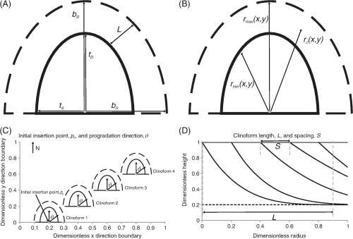
Figure 4 (A) A user specifies the length of the top (solid line) and base (dashed line) ellipses in depositional dip and strike directions (ts, tD, bs, bD; Table 1) relative to the clinoform origin. The surface representing the clinoform is created in the volume between the top and base ellipses. (B) At a point on the clinoform, the radius relative to the clinoform origin (black arrow, rc(x, y), the radius of the base ellipse (black arrow, rmax(x, y) and the radius of the top ellipse (black arrow, rmin(x, y) are calculated. (C) Plan view of four adjacent clinoforms. The user specifies the overall progradation direction of the clinoforms relative to north, as well as the coordinates of the initial insertion point PO. (D) Conceptual depositional-dip-oriented cross-section view of clinoforms. Clinoform spacing, S, is defined as the distance between the top truncation points of two adjacent clinoforms. Clinoform length, L, is defined as the distance between the top and base truncations by the user-specified bounding surfaces along a single clinoform.


The depositional processes acting at the shoreline control the plan-view shape and abundance of clinoforms and their associated heterogeneity.[9] Maps, satellite images, and aerial photographs of modern systems are used to make a first-order approximation of the distinct plan-view shape of clinoforms in different depositional environments (Figure 3), as described in the subsequent text, because there is a paucity of reliable data of this type from subsurface reservoirs and ancient analogs. This approximation assumes that the modern-day shape of a shoreline represents a snap-shot in time that mimics the geometry of clinoforms and associated depositional elements preserved in the stratigraphic record.[9] Mattson and Chan[41] assumed a simple radial geometry in plan view for fluvial-dominated deltaic clinoforms in the Ferron Sandstone Member outcrop analog, but this geometry is not universally applicable even as a first-order approximation. For example, wave-dominated strandplains are nearly linear in plan view (Figure 3A), wave-dominated deltas have broad arcuate forms (Figure 3B), and fluvial-dominated deltaic shorelines form distinct, lobate protuberances (Figure 3C) (e.g., Galloway[28]).
As the algorithm is generic, the user can specify the shape of an ellipse that approximates the plan-view geometry of clinoforms (Figure 4A). Using an ellipse, rather than a radial geometry, allows the user to specify a wide range of plan-view clinoform geometries using a simple function, depending on the interpreted environment of deposition and scale of shoreline curvature. Two ellipses are used: the top ellipse represents the shoreline at the clinoform top, and the base ellipse represents the maximum extent of the clinoform at its downlap termination on the underlying sea floor. The user defines the length of the top and base ellipses in depositional dip and strike directions (ts, tD, bs, bD; Figure 4B, Table 1) relative to the origin of the clinoform. The difference between the user-defined maximum extents of the top and base ellipses yields the clinoform length L (Figure 4D). The maximum extent of the top and base ellipses can then be defined as

and

The clinoform is generated in the volume between the top and base ellipses (Figure 4A, B). In this volume, the radius of each point on the clinoform, rc(x, y) (Table 1), is calculated relative to the clinoform origin (xorigin, yorigin), using

At each point on the clinoform, the radius of the top ellipse relative to the clinoform origin is calculated using

and the radius of the base ellipse using

To specify highly lobate plan-view clinoform geometry, characteristic of a fluvial-dominated delta (Figure 3C), the user specifies a larger value for the clinoform in the depositional dip direction, tD, than for the clinoform in the strike direction, tS. For a highly elongate or near-linear plan-view clinoform geometry, characteristic of a wave-dominated shoreline (Figure 3A, B), the user specifies a much larger value for the clinoform in the depositional strike direction, tS, than for the clinoform in the dip direction, tD. Data describing clinoform extent in depositional dip and strike directions can be extracted from published data on the dimensions of ancient shorelines or by analysis of their modern counterparts (e.g., tables 1, 2 in Howell et al.[9]).
| Parameter | Description | Min–Max Values | Units |
|---|---|---|---|
| tD | Length of top ellipse in depositional dip direction | 6100 | m |
| tS | Length of top ellipse in depositional strike direction | 4050 | m |
| L | Clinoform length | 60-495 | m |
| bD | Length of base ellipse in depositional dip direction (= tD + L) | 6160-6595 | m |
| bS | Length of base ellipse in depositional strike direction (= tS + L) | 4110-4545 | m |
| P | Shape function exponent | 2 | None |
| pO | Axis of progradation relative to bounding surfaces | 32% | None |
| θ | Clinoform progradation angle relative to north | 274 | ° |
| S | Clinoform spacing | 25 | m |
Cross-Sectional Clinoform Geometry[edit]
The shape and dip angle of a deltaic or shoreface clinoform in cross section is a function of modal grain size, proportion of mud, and the depositional process regime at the shoreline. In sandy, fluvial-dominated deltas, clinoforms have simple concave-upward geometries and steep dip angles (up to 15°)[4] (e.g., Figure 1). Similar geometries have been documented in sandy, tide-influenced deltas (dip angles up to 5°–15°).[42] Concave-upward clinoform geometry is also typical of sandy, wave-dominated deltas and strandplains, although the clinoforms have smaller dip angles (typically up to 1°–2°).[43][4] Clinoforms are consistently inclined paleobasinward down depositional dip; and, along depositional strike, they exhibit bidirectional, concave-upward dips if the delta-front was lobate in plan view (e.g., Willis et al.;[42] Kolla et al.;[44] Roberts et al.[34]) or appear horizontal if the shoreline was approximately linear (e.g., Hampson[45]). Clinoforms are usually truncated at their tops by a variety of channelized erosion surfaces formed during shoreline advance (e.g., distributary channels, incised valleys) and by channelized and/or planar transgressive erosion surfaces (tide and wave ravinement surfaces sense Swift[46]) associated with shoreline retreat. Consequently, most sandy shoreline clinoforms lack a decrease in depositional dip (rollover) near their tops, although this geometry is ubiquitous in larger, shelf-slope margin clinoforms (e.g., Steckler et al.[47]) and in the outer, muddy portion of compound deltaic clinoforms with a broad subaqueous topset that lies seaward of the shoreline (e.g., Pirmez et al.[48]).
Here, a geometric approach is used to represent the depositional dip cross-section shape of a clinoform with a dimensionless shape function, s(rc) (Figure 2E), such as a power law for concave-upward, sandy, shoreline clinoforms:

However, as the algorithm is generic, the mathematical expression of the dimensionless shape function is interchangeable so that other clinoform geometries can be represented; for example, a sigmoid function can be used to represent clinoforms in a larger, shelf-slope margin settings (e.g., Steckler et al.[47]). By combining the height function (equation 1), with the shape function (equation 7), the clinoform shape function, c(rc), is used to construct the shape of a clinoform surface:

By varying the exponent in the clinoform shape function, P, the user can increase or decrease the dip angle and change the shape of the clinoform (Figure 2E, Table 1). If a similar geometry is interpreted for each clinoform within a parasequence, because they are inferred to have formed under the influence of similar hydrodynamic and sedimentologic processes, then the same value of P (equation 7) can be applied to each clinoform modeled in the parasequence. Different values of P can be applied to distinct geographic regions of a parasequence in which clinoforms are interpreted to have different geometries (e.g., on different flanks of an asymmetric wave-dominated delta;[49][50]), provided that the bounding surfaces of these geographic regions have been defined (in the initial step of the method).
Spacing and Progradation Direction of Clinoforms[edit]
The clinoform-modeling algorithm allows the user to specify the main progradation direction of the clinoforms and to define the intervals along the progradation path at which clinoforms are generated (i.e., the clinoform spacing). The user specifies a progradation direction relative to north, θ (Figure 4C, Table 1), along which successive clinoforms are generated, which corresponds to the progradation path of the shoreline during clinoform deposition (plan-view shoreline trajectory of Helland-Hansen and Hampson[27]). The user also specifies the initial insertion point for the clinoforms, Po (Figure 4C). This provides flexibility in determining where to place the initial clinoform relative to the proximal model boundary. The spacing between each clinoform surface, S (Table 1), is also designated by the user. Clinoform spacing is defined as the distance between the top-truncation points of two successive clinoforms, and it determines the origin position, (xorigin, yorigin), of successive clinoforms (Figure 4D).
Stochastic Modeling of Clinoforms[edit]
Each of the input parameters described for the clinoform-modeling algorithm can be applied deterministically; however, many can also be applied stochastically (Table 1). If a reservoir model is created using an outcrop data set, it may be appropriate for the user to specify the parameter values for each clinoform. If a subsurface reservoir model is being created in which the parameter values are uncertain, the user can constrain a continuous probability distribution, such as a normal distribution, to assign values to each parameter. The user specifies the mean, standard deviation, and maximum and minimum values for the distribution. Values are then drawn at random from the distribution to assign values to the parameters.
Because many of the input parameters can be defined stochastically, one of the consequences of this aspect of the clinoform-modeling algorithm is that it is possible to generate complex geometries, such as cases in which clinoforms are observed to onlap against older clinoforms in the same parasequence. A combination of three factors is postulated to cause subtle changes in clinoform geometry and position, which combine to produce onlap in depositional-dip-oriented cross sections: (1) in fluvial-dominated deltas, distributary mouth bars and bar complexes have complex 3-D geometries that can shift along depositional strike as well as down depositional dip (e.g., Olariu et al.;[51] Wellner et al.[30]); (2) riverine sediment supply to delta-front clinoforms exhibits temporal and spatial variability that is related, at least in part, to downstream branching and switching of distributary channels as deltas advance (e.g., Wellner et al.;[30] Ahmed et al.[36]); and (3) clinoform geometries are locally modified by basinal processes such as waves and tides (e.g., Gani and Bhattacharya[33]).
To produce onlap and other subtle geometric features between successive clinoforms, the user can use the stochastic component of the clinoform-modeling algorithm to generate small variations in the parameter values of either or all of the following: progradation direction, θ; clinoform spacing, S; and clinoform length, L. If the parameters that define a clinoform cause it to be present below an earlier surface, it is truncated by the earlier surface to produce onlap. Application of the algorithm to (1) a rich, outcrop data set and (2) a sparse, subsurface data set is described in the examples in the following two sections.
Example 1: Ferron sandstone reservoir analog[edit]
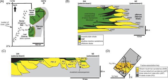
Figure 5 (A) Paleogeographic reconstruction of the Late Cretaceous Last Chance and Vernal delta systems of the Ferron Sandstone Member of the Mancos Shale in present-day Utah (after Cotter;[52] used with permission of Brigham Young University). The location of the Deveugle et al.[1] model (Figure 5D) and a regional cross section (Figure 5B) are highlighted. (B) Schematic regional cross section through the Last Chance delta system of the Ferron Sandstone Member and its eight-component shallow-marine tongues (termed “pararasequence sets,” using the nomenclature of Deveugle et al.,[1] and numbered PSS1 to PSS8), from southwest (paleolandward) to northeast (paleoseaward) (after Anderson and Ryer;[53] used with permission of AAPG). (C) Detailed cross section through the lowermost shallow-marine tongues (termed “parasequences,” using the nomenclature of Deveugle et al.,[1] and forming PSS1 in Figure 5B) and associated coastal-plain strata (after Garrison and Van den Bergh;[54] used with permission of AAPG). The tongue is subdivided into constituent parasequences (after Deveugle et al.[1]). Parasequence 1.6 is modeled in this study. (D) Distribution of facies-association belts at the top of parasequence 1.6, in the Deveugle et al.[1] model area in the Ivie Creek amphitheater. The area of the model constructed in this study (Figures 7, 8, 9 & 10) lies within the dashed lines.
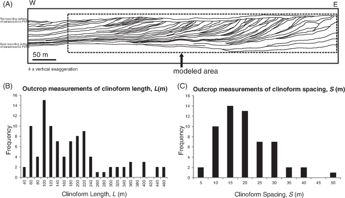
Figure 6 (A) Interpreted line drawing of clinoforms in parasequence 1.6 at the Junction Point section of Ivie Creek amphitheater (Figure 5D) (modified after Forster et al.[18]). Each clinoform bounds a mouth bar and equivalent delta-front deposits. Data from 104 clinoforms were collected to condition the clinoform-modeling algorithm. Frequency distributions of values measured from outcrop data for (B) clinoform length (Figure 4D), and (C) clinoform spacing (Figure 4D), which are used as input parameters in the clinoform-modeling algorithm (Table 2).


Geological Setting[edit]
Construction and fluid-flow simulation of models based on outcrop analogs is an established method for investigating geologic controls on subsurface reservoir performance (e.g., Ciammetti et al.;[55] White and Barton;[56] White et al.;[57] Jackson et al.;[11] Sech et al.;[5] Enge and Howell[12]). Here, the clinoform-modeling algorithm is used to build a reservoir model utilizing a high-resolution outcrop data set from the Ferron Sandstone Member, Utah, at a scale that is comparable to the interwell spacing (750 × 3000 m [2461 × 9843 ft] areally) in a typical hydrocarbon reservoir and captures several tens of clinoforms and their associated heterogeneities. Previously, Forster et al. [18] constructed 2-D flow-simulation models of the same outcrop analog via data-intensive, deterministic mapping of clinoforms and facies boundaries in cliff-face exposures. In contrast, our aim is to verify that the clinoform-modeling algorithm can produce realistic 3-D stratigraphic architectures that mimic rich outcrop data sets when conditioned to sparse input data that are typical in the subsurface. The scale of the model fills the gap between detailed but sparse 2-D core and well-log data and low-resolution but extensive 3-D seismic data.
The Ferron Sandstone Member of the Mancos Shale is located in east-central Utah. The unit was deposited during the Late Cretaceous (Turonian–Coniacian) on the western margin of the Western Interior Seaway and, in the study area, records the progradation of the Last Chance delta system from southwest (paleolandward) to northeast (paleoseaward)[52] (Figure 5A). These deltaic deposits form a basinward-thinning wedge that passes eastward into the offshore deposits of the Mancos Shale. The wedge contains either seven[58][59][60] or eight sandstone tongues,[53][54] such that one tongue is equivalent to a parasequence set of Deveugle et al.[1] (Figure 5B). A single delta-lobe deposit within the lowermost sandstone tongue is the focus of the study (bedset Kf-1-Iv[a] of Anderson et al.;[61] parasequence 1h of Garrison and Van den Bergh;[54] parasequence 1.6 of Deveugle et al.[1]) (Figure 5C, D). The delta-lobe deposit is fluvial dominated with low-to-moderate wave influence[59][54][62] and contains numerous, well-documented clinoforms in the exposures of the Ivie Creek amphitheater[63][64][61][18][12] (Figure 5D). Clinoform-related bedding geometries and facies distributions imply that clinoforms mapped by previous workers, and used as input data for the models presented below (Figure 6A, after Forster et al. [18]), bound clinothems equivalent to mouth bars (sensu Bhattacharya[29]). Subtle, apparently cyclic variations in clinoform spacing and dip angle probably define mouth-bar assemblages (sensu Bhattacharya;[29] “bedsets” sensu Enge et al.[65]). Smaller-scale lithologic variation at the scale of individual beds occurs between the mapped clinoforms and records incremental growth of a mouth bar because of varying water and sediment discharge through the feeder distributary channel. Deveugle et al.[1] used a high-resolution outcrop data set to build a reservoir-scale (7200 × 3800 × 50 m [23622 × 12467 × 164 ft]), surface-based model of the lower two tongues (parasequence sets) of the Ferron Sandstone Member. Clinoforms were not represented in the delta-lobe deposits (cf. parasequences) of the Deveugle et al.[1] model, and their surface-based model is used here as the context in which the clinoform-modeling algorithm should be applied.
Model Construction[edit]
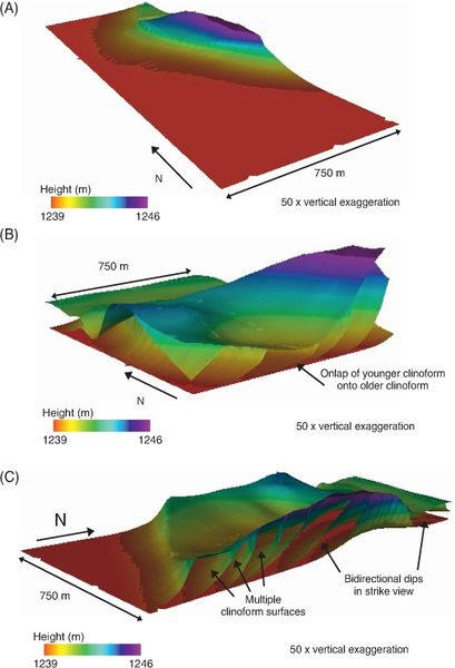
Figure 7 Surfaces generated by the clinoform-modeling algorithm for the model of part of parasequence 1.6 of the Ferron Sandstone Member (Figure 5C, D). (A) Single three-dimensional (3-D) surface representing a clinoform generated by the clinoform modeling algorithm. (B) 3-D dip cross section showing the concave-upward geometry of the clinoforms. (C) 3-D strike section of the model showing surfaces that exhibit bidirectional dips. Not all surfaces used in the model of part of the Ferron Sandstone Member (Figure 8) are shown.
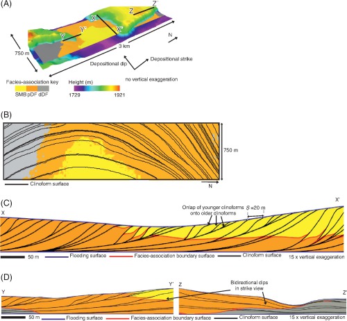
Figure 8 Surface-based model of part of parasequence PS1.6 of the Ferron Sandstone Member (Figure 5C, D), a fluvial-dominated delta lobe. (A) Three-dimensional view of the surface-based model, generated using bounding surfaces that were modified from the outcrop model of Deveugle et al.,[1] superimposed on a digital elevation map of the present day study area, with no vertical exaggeration and orientations of regional depositional dip and strike shown. (B) Plan-view section of model showing curved clinoforms, consistent with the geometry of fluvial-dominated delta lobes. (C) A two-dimensional (2-D) dip section and (D) a 2-D strike section through the model, showing details of the complex internal architecture. Red lines indicate facies boundaries, and blue lines indicate parasequence-bounding flooding surfaces. Black lines represent clinoforms. SMB = stream-mouth-bar; pDF = proximal delta-front; dDF = distal delta-front.


The top and base flooding surfaces of parasequence 1.6 were extracted from the model of Deveugle et al.[1] and served as the bounding surfaces used in the clinoform algorithm (Figure 2). The surfaces were cropped to cover a model area of 750 × 3000 m (2461 × 9843 ft) in the Ivie Creek amphitheater (Figure 5D). Additional surfaces representing the boundaries between facies associations from the model of Deveugle et al.[1] were also extracted and similarly cropped; these define the distribution of facies associations present in each rock volume bounded by two clinoforms (i.e., clinothem) (cf. table 1 in Deveugle et al.[1]). From distal to proximal, the modeled facies associations are prodelta mudstone (PD), distal delta-front heteroliths (dDF), proximal delta-front sandstones (pDF), and stream-mouth-bar sandstones (SMB) (Figure 5D). Where facies associations pinch out, the facies association boundary surfaces were adjusted to coincide throughout the remainder of the model volume with either the top or base parasequence bounding surface. This ensures that the surface is defined across the entire model volume and is suitable for gridding.[11] There are no faults within the model volume of 750 × 3000 × 6 m (2461 × 9843 × 20 ft). In a final step, isochore maps were generated between the top and base flooding surfaces and between facies association boundary surfaces and the base flooding surface. The base bounding surface was flattened, to mimic clinoform progradation over a flat, horizontal sea floor, and isochore maps were used to modify the geometries of the top bounding surface and facies association boundary surfaces above this horizontal base surface. As a result of flattening on the base bounding surface, the bounding surfaces from the existing model of Deveugle et al.[1] have been modified.
The parameters used to insert clinoforms into the model volume are summarized in Table 2. The delta lobe in parasequence 1.6 is approximately 8.1 km (5.03 mi) wide and 12.2 km (7.58 mi) long, giving a plan-view aspect ratio of 0.7,[1] comparable to values for lobes of the Pleistocene Lagniappe delta (after data in Kolla et al.;[44] Roberts et al.[34]) and the modern Wax Lake Delta lobe (after data in Wellner et al.[30]) (Figure 3C). These dimensions were likely smaller during the growth of the delta lobe, and it is assumed here that the lobe initiated with dimensions (tD, ts) that were a third of those of the final preserved delta lobe, consistent in areal proportions to a single mouth-bar assemblage or jet-plume complex in the modern Wax Lake Delta lobe (after data in Wellner et al.[30]). The length, L, and spacing, S, of clinoforms in depositional dip cross section were extracted from the bedding-diagram interpretations of Forster et al. [18] (Figure 6A), clinoform length and dip statistics of Enge et al.,[65] and the LIDAR data used to create the model of Enge and Howell.[12] A database of clinoform lengths, dips, and spacings was compiled from these data sources, yielding frequency distributions from which the geometry or spatial arrangement of clinoforms that bound mouth-bar clinothems (sensu Bhattacharya[29]), or a trend in these parameters, can be extracted (Figure 6B, C). The clinoform-modeling algorithm was used to build 31 clinoforms in the modeled volume of parasequence 1.6 (Figure 7). For simplicity, clinoform spacing is fixed at 25 m (82 ft), which is the average value observed at outcrop (Figure 6C). Heterogeneity at bed scale is recognized to be present but is not explicitly captured by surfaces in the model; rather, the effective petrophysical properties assigned to the facies associations (particularly the ratio of vertical-to-horizontal permeability) are modified to account for these.[11][1][26] A constant value of 2 was assigned to the clinoform shape-function exponent, P (Figure 2E), to ensure that the clinoform dip angle is always in the range extracted from the data of Enge et al.[65] The initial clinoform insertion point, Po (Figure 4C), was qualitatively matched with a plan-view map of facies association belts at the top of parasequence 1.6 (Figure 5D). The overall progradation direction for the clinoforms (θ) was assigned an azimuth of 274° relative to north, which corresponds to the interpreted progradation direction of the delta lobe in parasequence 1.6.[1] In a subsequent step, the facies association boundary surfaces extracted from the model of Deveugle et al.[1] were used to create facies association zones within each clinothem. Application of the clinoform-modeling algorithm yields a surface-based model measuring 750 × 3000 × 6 m (2461 × 9843 × 20 ft), which contains 95 surfaces: the top- and base-parasequence bounding surfaces, 31 clinoforms, and 62 facies-association boundary surfaces (Figure 8).
A cornerpoint gridding scheme in which variations in facies architecture are represented by variations in grid architecture was used.[56][66][5] The grid has vertical pillars with a constant spacing of 20 m (66 ft) in x and y (horizontal) directions. Grid layering in the z (vertical) direction within each facies-association zone conforms to the underlying clinoform surface, so layers are parallel to, and build up from, the underlying clinoform. Grid layers have a constant thickness of 0.2 m (0.66 ft); however, each facies-association zone is gridded separately, and the grid layers pinch out against facies-association boundaries and parasequence-bounding flooding surfaces. This gridding approach was used by Sech et al.;[5] it ensures that the grid layering conforms to the architecture of the clinoform surfaces, preserving their dip and geometry, and captures facies association boundaries (Figure 9). Where a grid layer pinches out, the grid cells have zero thickness and are set to be inactive in flow simulations. These zero-thickness cells are bridged using nonneighbor connections so that they do not act as barriers to flow. The chosen cell size of 20 × 20 × 0.2 m (66 × 66 × 0.66 ft) yields a total of approximately 5 million cells, of which 140,000 (2.6%) are active. Because the number of active grid cells is small, fluid-flow simulations can be performed on the grid without upscaling.
In the final step before fluid-flow simulation, the grid cells were populated with petrophysical properties from a mature subsurface reservoir analog (table 1 of Deveugle et al.[1]). Petrophysical properties were assigned to each facies association, which typically have permeabilities that differ by approximately one order of magnitude from their overlying or underlying neighbor. In a separate step, transmissibility multipliers are assigned along the base of the grid cells in the layer directly above each clinoform surface to represent baffles and barriers to fluid flow along clinoforms in a geometrically accurate and efficient way. The transmissibility multipliers were assigned using a stochastic technique that decreases the probability of barriers being present along the upper part of the clinoform. This aspect of modeling is discussed in greater detail in a companion article.[26]
Geologic Model Results[edit]

We begin by investigating the ability of the clinoform-modeling algorithm to generate realistic stratal geometries from the Ferron Sandstone Member outcrops. Visual inspection of the algorithm-generated model against outcrop photo pans (Figure 1) and bedding diagram interpretations (Figure 6A) reveals a close correspondence between key geometric aspects of the observed data and concepts reproduced in the model, as outlined below.
A single delta lobe is present in the model and extends beyond the model volume (Figures 5D, 8A). As a result, clinoforms are larger in their depositional dip and strike extent (tD and ts, respectively; Table 2) than the model area, and they form arcs in plan view in the model (Figure 8B). This plan-view geometry is consistent with the approximately lobate plan-view geometries of clinoforms in fluvial-dominated deltas (Figure 3C). The clinoform-modeling algorithm generates the concave-upward clinoform geometry observed at the outcrop (Figures 7B, 8C), while honoring the topography of the parasequence bounding surfaces. The variation in topographic elevation of the modeled parasequence (Figures 7, 8) is attributed to postdepositional compaction. In a depositional strike cross section of the clinoform-bearing model, the algorithm produces bidirectional concave-upward dips (Figures 7C, 8D) that are consistent with delta-front bodies that are lobate in plan view (e.g., Willis et al.;[42] Kolla et al.;[44] Roberts et al.[34]). Additionally, the model contains stratal geometries observed at the outcrop, such as onlap and downlap of younger clinoforms on to older clinoforms (Figures 7B, 8C). The clinoform-modeling algorithm also produces clinoforms that are consistently distributed in the same orientation as those in the observed delta-lobe deposits and its interpreted plan-view progradation direction (Figures 5A, 8B). Facies proportions in the model are 8% SMB sandstones, 50% pDF sandstones, 31% dDF heteroliths, and 11% PD mudstone. Using porosity values that are characteristic of these facies associations in analogous reservoirs (Table 3), the volume of oil in place in the model is 7.1 million bbl. The clinoform-bearing model is now used to investigate the impact of heterogeneities associated with clinoforms on fluid flow during waterflooding within this fluvial-dominated deltaic parasequence.
| Properties | Value | Units |
|---|---|---|
| Reservoir Properties | ||
| Reservoir pressure (Pr) | 100 | bar |
| Oil–water contact (OWC) | 600 | m |
| Top | 1253 | m |
| Base | 1246 | m |
| Fluid Properties | ||
| Oil viscosity (μo) | 0.7 | cp |
| Oil density (ρo) | 650 | kg/m3 |
| Oil compressibility (co) | 10-4 | 1/bar |
| Oil formation volume factor (Bo) | 1.00000009 | (rm3/sm3) |
| Water viscosity (μw) | 0.3 | cp |
| Water density (ρw) | 950 | kg/m3 |
| Water compressibility (cw) | 10^-5 | 1/bar |
| Water formation volume factor (Bw) | 1 | (rm3/sm3) |
| Rock Properties | ||
| Porosity (⊘) of prodelta mudstone (PD) facies association | 0 | % |
| Horizontal (kh) and vertical permeability (kv) of PD facies association | 0, (kh), 0 (kv) | md |
| Porosity (⊘) of distal delta-front heteroliths (dDF) facies association | 18 | % |
| Horizontal (kh) and vertical permeability (kv) of dDF facies association | 71 (kh), 7 (kv) | md |
| Porosity (⊘) of proximal delta-front sandstones (pDF) facies association | 27 | % |
| Horizontal (kh) and vertical permeability (kv) of pDF facies association | 433 (kh), 325 (kv) | md |
| Porosity (⊘) of stream-mouth-bar sandstones (SMB) facies association | 28 | % |
| Horizontal (kh) and vertical permeability (kv) of SMB facies association | 1793 (kh), 1614 (kv) | md |
| Rock compressibility for all facies associations (cr) | 10-12 | 1/bar |
Production Strategy[edit]
Waterflooding was simulated using conventional black oil simulation software, using a line drive of four vertical injector wells and six vertical producer wells (Figure 10A). The producer and injector wells were spaced 750 m (2461 ft) apart, with water being injected down the local depositional dip, from east to west. Oil production and water injection were set to maintain a group target production rate over 20 yr of 175 S m3/day (1100 bbl/day), a minimum bottom hole pressure constraint of 50 bars (725 psi) for each production well, and a maximum bottom hole pressure constraint of 150 bars (2175 psi) for each injection well. Further information on reservoir properties is summarized in Table 3. Heterogeneity along clinoforms is specified in terms of the percentage of each clinoform surface that acts as a barrier to flow. The volume of the barriers along clinoforms is negligible, so they have little impact on the volume of oil in place. Two simulations were completed in which (1) clinoforms are not associated with barriers to flow (0% barrier coverage along clinoforms) and (2) clinoforms are associated with significant barriers to flow (90% barrier coverage along clinoforms; Figure 10B). All other parameters remain fixed between the simulations. In a companion article, Graham et al.[26] apply the clinoform-modeling algorithm to build a range of models to investigate the impact of a broader range of uncertainties in clinoform parameters, such as clinoform spacing and barrier coverage, on hydrocarbon recovery in the context of uncertain geologic parameters and engineering decisions.
Simulation Results[edit]

When clinoforms are not associated with barriers to flow, they have little impact on production (Figure 10C); however, if barriers occupy 90% of the clinoform surfaces, then their impact on recovery is significant. Models that omit barriers to flow along clinoforms can overestimate recovery by up to 36% (cf. Figures 10C, D; 11A), consistent with previous simulation studies of the Ferron Sandstone Member that found barrier-lined clinoforms reduced hydrocarbon recovery by several tens of percent.[10][12] Reduced recovery is caused by decreased sweep efficiency as each clinothem becomes hydraulically separated from its neighbors. Consequently, significant oil is bypassed in the reservoir, particularly beneath barriers along clinoforms and at the toe of each clinothem (Figure 10D). Increased reservoir compartmentalization also means that the target oil production rate cannot be met; and, as a result, models that include barriers along clinoforms produce significantly lower volumes of oil per day (Figure 11B). Enge and Howell[12] also found that including barriers along clinoforms in reservoir models of the Ferron Sandstone Member increased reservoir compartmentalization.
Finally, models that include barriers along clinoforms have earlier water breakthrough than models that lack barriers along clinoforms (Figure 11). Including barrier-lined clinoforms increases the tortuosity of flow pathways because the fluids can only move between clinothems by exploiting the gap in the barriers at the top of each clinoform. However, as the number of potential flow pathways is decreased by including barriers to flow along clinoforms, the injected water exploits the pathways between the injectors and producers faster, which leads to earlier water breakthrough. Similar results were obtained in clinoform-bearing models of a wave-dominated shoreface system .[11]
Although barriers to flow along clinoforms are thin (<20 cm [<8 in.]) and constitute only a small proportion of the overall model volume, they significantly affect permeability architecture, sweep pattern and simulated oil recovery. Therefore, under certain displacement conditions, it is important to include barriers associated with clinoforms in simulation models of analogous shallow-marine reservoirs. The clinoform-modeling algorithm supports the results of previous studies of the Ferron Sandstone Member and demonstrates an efficient new method to incorporate multiple, geometrically realistic clinoforms into simulation models.
Example 2: Troll west reservoir sector model[edit]

Geological Setting[edit]
The clinoform-modeling algorithm is now applied to construct a model of the Upper Jurassic Sognefjord Formation reservoir in a fault-bounded sector of the Troll Field, offshore Norway (Figure 12A, B). The Troll Field is a supergiant gas field that initially hosted about 40% of the total gas reserves on the Norwegian continental shelf and still contains ca. 1000 x 109 S m3 (35 tcf) of gas.[71] The western and eastern parts of the Troll Field accumulation occur in different structures, Troll West and Troll East. The Sognefjord Formation is interpreted to record deposition in a mixed fluvial-, tide-, and wave-influenced delta system.[69][72] The formation is up to 170 m (558 ft) thick in the Troll Field and consists of five, vertically stacked regressive–transgressive successions bounded by major flooding surfaces (informally referred to as the 2-, 3-, 4-, 5- and 6-series in the reservoir; Figure 12C).[69] Each regressive–transgressive succession exhibits internal stratigraphic variability across the lateral extent of the reservoir, such that it can be interpreted as a sequence with constituent systems tracts and parasequences.[69] The reservoir volume to be modeled contains seven, vertically stacked parasequences. The lower parasequences were deposited by regression of wave-dominated delta-fronts, whereas the upper parasequences comprise more tide-influenced delta-front deposits.[69]
Reservoir zones in the Troll West accumulation are defined by alternating layers of fine-grained, micaceous sandstone and coarse-grained sandstone (informally referred to as m sands and c sands, respectively). The coarse-grained sandstones have higher porosity and permeability (hundreds to thousands of millidarcys) than the fine-grained, micaceous sandstones (tens to hundreds of millidarcys).[70][69] Each couplet of fine-grained, micaceous sandstone and overlying coarse-grained sandstones corresponds to the lower and upper part of a single delta-front parasequence.[69] The 3-D seismic data image laterally extensive (up to 30 km [19 mi] along depositional strike), near-linear, north-northeast–south-southwest-trending clinoforms that dip west-northwestward at 1.5°–4°.[69][72] The structure of the Troll West reservoir is defined by two rotated fault blocks that formed after reservoir deposition, and the reservoir is further segmented by smaller postdepositional faults that trend west-northwest–east-southeast to north-northwest–south-southeast[69] (Figure 12B).
Troll West contains a thin oil column (11–26 m [36–85 ft]) that is exploited through the use of horizontal wells,[69] the productivity of which is sensitive to the ratio of vertical-to-horizontal permeability (cf. Joshi[73]). This ratio is predicted to be influenced by the calcite-cemented concretionary beds that are abundant in the Sognefjord Formation.[74][75][76] These are present within delta-front parasequences, which are seismically imaged as clinoform sets, and along their bounding flooding surfaces.[70][77][69][78][72] The Jurassic Bridport Sand Formation, a close sedimentologic analog present onshore United Kingdom, contains similarly abundant calcite-cemented concretionary beds. These are observed at the outcrop to be laterally extensive (>80% areal coverage) along bedding planes and in a producing subsurface reservoir; their presence is marked by breaks in pressure and fluid saturation within seismically imaged clinoform sets.[79][80] Thus it appears probable that permeability barriers and baffles in the form of calcite-cemented concretionary layers occur along clinoforms in the Troll Field reservoir and could influence drainage patterns and recovery from the thin oil zone;[70] this may have been recognized previously and shown to impact on well test interpretations.[81][82] However, to date, the heterogeneity associated with clinoforms has not been explicitly included in reservoir or flow-simulation models of the Sognefjord Formation in the Troll Field. Dilib et al.[83] created a sector model of the Sognefjord Formation (dimensions: 3200 × 750 × 150 m [10,499 × 2461 × 492 ft]) to investigate production optimization using intelligent wells for a range of uncertainty in geologic parameters and their model, extracted and refined from the existing full field geological model, was used here as the context in which to apply the clinoform-modeling algorithm.
Model Construction[edit]

The stratigraphic framework of the reservoir model is defined by flooding surfaces that bound seven parasequences. The bounding surfaces are offset by two postdepositional faults that are oriented northwest–southeast across the model volume. The faulted parasequence-bounding flooding surfaces were extracted from the existing reservoir model.[83] The faulted parasequence boundaries were used to construct the final Troll West sector model but, as a quality control step for applying the clinoform-modeling algorithm, these boundaries were adjusted so that they were horizontal. Each parasequence also contains a surface that represents the facies-association boundary between m sands below and c sands above; these surfaces were extracted from the model of Dilib et al.[83] and are laterally continuous across the clinoforms modeled here, because they were extracted from a model that omits clinoforms. Consequently, facies interfingering across clinoforms is not captured here, and this may further increase the impact of modeling clinoforms on flow.[11] The facies-association boundary surfaces were adjusted to remove the effects of faulting in the same way as the flooding surfaces. Additionally, where facies associations pinch out, the facies association boundary surfaces are adjusted to coincide throughout the remainder of the model volume with the top parasequence bounding surface. This procedure created flooding surfaces and facies-association boundaries in the model that mimic their depositional geometries, which were used as a reference framework to validate that the clinoform geometries and distributions applied later using the faulted parasequence-bounding surfaces are consistent with geologic concepts.
Table 4 shows the parameters used in the clinoform-modeling algorithm. To honor the nearly linear plan-view geometry of clinoforms observed in seismic data (figures 3, 12 in Dreyer et al.[69]), a width for the top-clinoform ellipse (ts) that is far greater than the depositional-dip extent of the bounding surfaces in the model area (3200 m [10,499 ft]) was defined; the top-clinoform ellipse length tD is half of ts, to give a plan-view aspect ratio of 2 (cf. wave-dominated shoreface systems in Howell et al.[9]). Seismically resolved clinoform dip values of 1.5°–4°[69][72] were used in conjunction with the estimated parasequence thickness to calculate clinoform length (L) using simple trigonometry. As there are only a small number of seismically resolved clinoforms in a few paleogeographic locations and within a few stratigraphic levels to extract clinoform length, a normal distribution based on the extracted data was generated (Figure 13A), and values were then drawn at random from this distribution to populate the model volume (Figure 13A). Finally, the premodeling lengths were compared with the seismically resolved clinoforms[69] to validate that the algorithm-generated lengths are reasonable. Similarly, the horizontal spacing of seismically resolved clinoforms (figures 3, 12 in Dreyer et al.[69]) was used to generate a normal distribution of values for clinoform spacing, S (Figure 13B), and values were drawn at random from this distribution to populate the model volume (Figure 13B). The resulting values of clinoform length and spacing are consistent with those observed at the outcrop for other wave-dominated shorelines (e.g., Hampson;[45] Sech et al.[5]) (Figure 13). A value of 2 was used for the exponent in the clinoform shape function (defined by P in equation 8), as this gives a good match to the seismically resolved clinoforms; and, furthermore, it was assumed that a similar geometry is shared by clinoforms in all parasequences in all locations throughout the model volume, consistent with observations of seismically resolved clinoforms over similar-size volumes.[72] Although, P has the same value as used in the Ferron Sandstone Member example, L values in the Troll Field sector model are larger (Figure 13A, Table 4) such that clinoform dip angles are shallower, consistent with the seismically resolved clinoforms.[69][72] As a first step, the insertion point of the first clinoform (Po) was arbitrarily selected in the center of the proximal model boundary, and consistent west-northwest progradation of clinoforms[69][72] was used to define a θ of 320°. The facies-association boundary surfaces extracted from the model of Dilib et al.[83] were then used to create zones of m sands and c sands within each clinothem. The application of the clinoform-modeling algorithm yields a model containing 100 clinoforms. A visual quality control check was then performed to ensure that the clinoforms produced by the algorithm are consistent with the geologic concepts of the model (e.g., clinoform spacing, dip, length) in the absence of postdepositional faults.
| Parameter | Description | Minimum–Maximum Values | Units |
|---|---|---|---|
| tD | Length of top ellipse in depositional dip direction | 3000 | m |
| tS | Length of top ellipse in depositional strike direction | 6000 | m |
| L | Clinoform length | 150–900 | m |
| bD | Length of base ellipse in depositional dip direction (= tD + L) | 3150–3900 | m |
| bS | Length of base ellipse in depositional strike direction (= tS + L) | 6150–6900 | m |
| P | Shape function exponent | 2 | None |
| pO | Axis of progradation relative to bounding surfaces | 50 | None |
| θ | Clinoform progradation angle relative to north | 320 | ° |
| S | Clinoform spacing | 105–390 | m |
After this validation, the clinoform-modeling algorithm was applied with the same parameters (Table 4) but using the faulted parasequence-bounding flooding surfaces and the faulted facies-association boundary surfaces. The resulting surface-based model contains clinoforms with geometries and distributions that reflect present-day reservoir structure, measures approximately 3200 × 750 × 150 m (10,499 × 2461 × 492 ft), and contains 215 surfaces: the 8 top and base parasequence bounding surfaces, 100 clinoform surfaces, and 107 facies-association-boundary surfaces between clinoform pairs. A hybrid gridding method is used, because previous work shows that this approach better captures the movement of gas and water in the vicinity of a horizontal production well located in a thin oil rim.[84] The areal grid resolution of the model is fixed (50 × 25 m [164 × 82 ft]), but the vertical resolution varies. In the gas cap and aquifer, the vertical layering is stratigraphic, conforming to the flooding surfaces that bound the parasequences and with a single grid layer representing each facies association zone. In an interval of the reservoir that contains the oil column, from 3 m (10 ft) above the gas–oil contact (GOC) to 3 m (10 ft) below the oil–water contact (OWC), the grid is horizontal and regular, with finer layering (0.25–2 m [0.82–7 ft]) parallel to the initial GOC and OWC.[83] Very fine grid resolution is required to capture the geometry of clinoforms in this regular, orthogonal part of the grid. For the model to be suitable for flow simulation, it is not possible to have this level of grid resolution everywhere in the model. Petrophysical properties were assigned by facies association in a similar manner to the model of the Ferron Sandstone Member reservoir analog. Clinoform-related heterogeneity was incorporated in flow-simulation models by using transmissibility multipliers along clinoform surfaces, where a trend was used to enforce greater continuity and extent of heterogeneity in the m sands that lie above the lower part of each clinoform. A different approach was used to model the clinoform-controlled heterogeneity than for the Ferron Sandstone Member model, because part of the grid is horizontal and regular. Transmissibility multipliers representing the heterogeneity along clinoforms are placed in the cells adjacent to the clinoform surface in the orthogonal part of grid around the oil rim. As the orthogonal grid is very fine, this approach honors the geometry of the clinoform surfaces.
Geologic Model Results[edit]
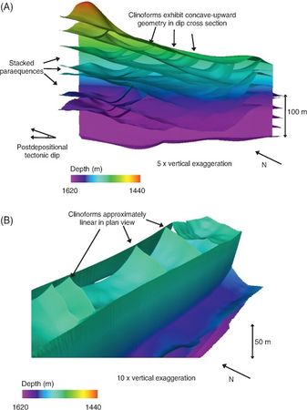
Figure 14 Surfaces generated by the clinoform-modeling algorithm for the Troll sector model. (A) Three-dimensional (3-D) dip cross section of clinoforms in the model demonstrating their concave-upward geometry. (B) 3-D view of clinoforms in the model showing close to linear clinoforms in plan view within fault-bounded compartment. Not all surfaces used in the Troll sector model (Figure 15) are shown.
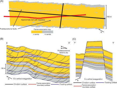
Figure 15 (A) Plan-view facies-association map through the uppermost parasequence of the Sognefjord Formation in our Troll West sector model, showing the location of compartmentalizing faults and a horizontal well. Cross sections along (B) depositional dip and (C) depositional strike, showing bounding flooding surfaces (blue), surfaces representing facies-association boundaries (red), and clinoforms generated by the modeling algorithm (black) for all parasequences in the model volume.


The clinoforms incorporated into the Troll sector model show similar geometries and spacing to those that are seismically resolved in the Sognefjord Formation.[69][72] The clinoforms are linear in plan view over the small (750 m [2461 ft]) depositional-strike extent of the model (Figure 14B), consistent with the interpreted plan-view geometries of wave-dominated shoreface systems (Figure 3A),[9] consistently prograde west-northwestward (θ = 320°), as established through 3-D seismic data,[69][72] and have the concave-upward geometry observed in seismic dip sections through the Sognefjord Formation[69][72] (Figures 14A, 15B). In depositional strike cross section, the algorithm produces near-horizontal clinoform geometries, consistent with seismically resolved clinoforms[69][72] (Figure 15C). The stochastic component of the clinoform-modeling algorithm distributes clinoforms with cross-sectional geometries and spacings (Figures 14A, 15B) that are consistent with outcrop studies of wave-dominated deltas[45][5] (Figure 13) and honor the sparse subsurface data. In contrast to the Ferron Sandstone Member example, the Troll West sector model does not contain subtle clinoform geometries, such as onlap and downlap of younger clinoforms on to older clinoforms (Figures 14A, 15B). Such features are below the resolution of the seismic data used to extract the parameters that were used in the algorithm. The clinoforms are also faulted in the same way as the parasequence-bounding flooding surfaces (cf. Figures 2A, 15C).
Production Strategy[edit]

The clinoform-bearing Troll West sector model was then used to simulate production through gas expansion and aquifer influx using a 2600 m (8530 ft) long horizontal well, placed 2 m (7 ft) above the initial OWC (Figures 15A, 16A). The well is controlled by maximum gas production rate, minimum oil production rate, and minimum bottom-hole-pressure constraints. Reservoir, rock, and fluid properties are summarized in Table 5. Similar to the Ferron Sandstone Member example, the presence of permeability barriers along clinoforms was modeled using transmissibility modifiers and specified in terms of the percentage of each clinoform surface that acts as a barrier to flow. Two simulations of the Troll Field sector model were conducted in which (1) clinoforms are not associated with barriers to flow (0% barrier coverage along clinoforms) and (2) clinoforms are associated with significant barriers to flow (90% barrier coverage along clinoforms, Figure 16B). All other parameters remain fixed between the simulations.
Simulation Results[edit]

The presence of barriers along 90% of the area of each clinoform surface significantly alters the movement of fluids in the reservoir by increasing the tortuosity of flow pathways. As a result, gas breakthrough is later when calcite-cemented barriers are present along clinoforms (30 vs. 15 days, Figure 17C), and oil production remains at plateau for longer (30 vs. 15 days, Figure 17A). However, after gas breakthrough, the rate of oil production rapidly falls below that for the case lacking calcite-cemented barriers (Figure 17A). Water cut is significantly lower for the model containing calcite-cemented barriers throughout production (Figure 17B). The calcite-cemented barriers along clinoforms prevent lateral movement of oil and the upward movement of water from the aquifer to the well (Figure 16D) but have a less significant effect on the downward movement of more mobile gas. As a result, the gas:oil ratio increases for production in the model containing calcite-cemented barriers along clinoforms. Most importantly, the recovery of oil could be overestimated by up to 14% if calcite cements associated with clinoforms were omitted from the reservoir model (Figure 17D; cf. Figure 16C, D); this is consistent with the results of Jackson et al.,[11] which showed that omitting clinoforms from wave-dominated shoreface systems could lead to overprediction of hydrocarbon recovery.
Discussion[edit]
We have described the conceptual and mathematical basis of a modeling algorithm to generate surface-based reservoir models that include clinoforms, and demonstrated its application using (1) a deterministic approach in which a rich, high-resolution data set is available (Ferron Sandstone Member outcrop analog) and (2) a stochastic element where the data are sparse (Sognefjord Formation, Troll Field sector).
Several previous studies of the Ferron Sandstone Member have incorporated clinoforms in flow simulation models using a combination of object-based methods to place barriers along clinoforms[10] or deterministic methods to map clinoforms.[9][12] Although these studies have demonstrated that, under certain displacement conditions, it is important to include clinoforms in models of shallow-marine reservoirs, it is not clear how these models could be applied in the subsurface or at the full-field scale. Other studies have indicated that surfaces should be used to incorporate clinoforms into reservoir models, as surfaces are much less computationally expensive to generate and manipulate than large 3-D geocellular grids.[11][5][12][85] These deterministic approaches are appropriate for modeling clinoforms that are tightly constrained by outcrop data but do not allow flexibility in conditioning clinoform geometry and distribution to sparser data sets with a large degree of uncertainty.
Our results support previous work in demonstrating that it is important to include clinoforms in models of shallow-marine reservoirs to accurately predict fluid-flow patterns and hydrocarbon recovery. However, the work presented here differs from previous modeling investigations in providing a generic method of incorporating clinoforms with geologically realistic geometries and spacing into models of shallow-marine reservoirs. The algorithm can be also be applied at a variety of lengthscales, as demonstrated in Graham et al.,[26] in which a reservoir scale model that comprises multiple stacked parasequences is used to investigate the impact of clinoforms under geologic uncertainty and reservoir engineering decisions.
We recognize that the algorithm does not explicitly incorporate every clinoform that may be present, but instead provides a mechanism to include clinoforms at a level of stratigraphic detail defined by the user, based on a combination of stratigraphic understanding, available data, and computing resources. Nor does the algorithm represent the detailed geometry of clinoforms, as may be possible using process-based forward numerical models (e.g., Edmonds and Slingerland;[19] Geleynse et al.[20]). However, there are uncertainties in the values of input parameters to use in process-based models, and these parameters cannot be easily extracted from outcrop analog or subsurface data sets. There are also no explicit relationships between the input parameters for process-based models and the parameters that describe the geometries of clinoforms produced, such as clinoform length, spacing, or width. Process-based models are also difficult to condition to available data and require large computational times, which make them less feasible for modeling a range of realizations. The clinoform-modeling algorithm presented here provides a flexible and efficient method for incorporating multiple clinoforms with realistic geometries into models of shallow-marine reservoirs.
The impact of clinoforms on flow also has implications for history matching reservoir models to production data. If the underlying geologic model has omitted clinoforms and is not representative of the reservoir, then history matching will fail to produce reliable models for accurate forecasting future production. The clinoform-modeling algorithm allows multiple surface-based, clinoform-bearing models to be generated rapidly to investigate uncertainty in reservoir characterization and to develop production strategies to mitigate this uncertainty. The algorithm can thus be used in conjunction with other modeling tools and techniques as a basis to inform fast decision making in reservoir management.
Conclusions[edit]
A surface-based clinoform-modeling algorithm has been developed as a tool for rapidly incorporating clinoforms into models of shallow-marine reservoirs. The algorithm is flexible and can be used in different shallow-marine environments through the user specifying a small number of input parameters.
The clinoform-modeling algorithm has been demonstrated using two different approaches and data sets: (1) a rich, high-resolution outcrop data set from a fluvial–deltaic reservoir analog (Cretaceous Ferron Sandstone Member, Utah), within which numerous clinoforms were modeled deterministically, and (2) a sparse subsurface data set from a sector of a subsurface reservoir (Jurassic Sognefjord Formation, Troll Field, Norwegian North Sea), within which numerous clinoforms were modeled stochastically. In both applications, geometrically realistic clinoforms were incorporated into existing reservoir models.
Finally, the clinoform-modeling algorithm allows clinoform geometry to be retained efficiently for fluid-flow simulation. Regardless of whether production is via vertical or horizontal wells or driven by waterflooding or by gas cap expansion and aquifer influx, it was found that omission of barriers to flow along clinoforms can lead to poor prediction of fluid movement and hydrocarbon recovery. Barriers to flow along clinoforms reduced hydrocarbon recovery on the order of 10%–20% in both cases, compared to the models that omitted clinoforms.
References[edit]
- ↑ 1.00 1.01 1.02 1.03 1.04 1.05 1.06 1.07 1.08 1.09 1.10 1.11 1.12 1.13 1.14 1.15 1.16 1.17 1.18 1.19 1.20 Deveugle, P. E. K., M. D. Jackson, G. J. Hampson, M. E. Farrell, A. R. Sprague, J. Stewart, and C. S. Calvert, 2011, Characterization of stratigraphic architecture and its impact on fluid flow in a fluvial-dominated deltaic reservoir analog: Upper Cretaceous Ferron Sandstone Member, Utah: AAPG Bulletin, v. 95, no. 5, p. 693–727, doi: 10.1306/09271010025.
- ↑ Barrell, J., 1912, Criteria for the recognition of ancient delta deposits: Geological Society of America Bulletin, v. 23, no. 1, p. 377–446, doi: 10.1130/GSAB-23-377.
- ↑ Rich, J. L., 1951, Three critical environments of deposition, and criteria for recognition of rocks deposited in each of them: Geological Society of America Bulletin, v. 62, no. 1, p. 1–20, doi: 10.1130/0016-7606(1951)62[1:TCEODA]2.0.CO;2.
- ↑ 4.0 4.1 4.2 Gani, M. R., and J. P. Bhattacharya, 2005, Lithostratigraphy versus chronostratigraphy in facies correlations of Quaternary deltas: Application of bedding correlation, inL. Giosan, and J. P. Bhattacharya, eds., River deltas—Concepts, models and examples: SEPM Special Publication 83, p. 31–47.
- ↑ 5.0 5.1 5.2 5.3 5.4 5.5 5.6 5.7 5.8 5.9 Sech, R. P., M. D. Jackson, and G. J. Hampson, 2009, Three-dimensional modeling of a shoreface-shelf parasequence reservoir analog: Part 1. Surface-based modeling to capture high resolution facies architecture: AAPG Bulletin, v. 93, no. 9, p. 1155–1181, doi: 10.1306/05110908144.
- ↑ 6.0 6.1 Wehr, F. L., and L. D. Brasher, 1996, Impact of sequence-based correlation style on reservoir model behaviour, lower Brent Group, North Cormorant field, UK North Sea, inJ. A. Howell, and J. A. Aitken, eds., High resolution sequence stratigraphy: Innovations and applications: Geological Society, London, Special Publication 104, p. 115–128.
- ↑ 7.0 7.1 Ainsworth, B. R., M. Sanlung, and S. T. C. Duivenvoorden, 1999, Correlation techniques, perforation strategies, and recovery factors: An integrated 3-D reservoir modeling study, Sirikit field, Thailand: AAPG Bulletin, v. 83, p. 1535–1551.
- ↑ Dutton, S. P., B. J. Willis, C. D. White, and J. P. Bhattacharya, 2000, Outcrop characterization of reservoir quality and interwell-scale cement distribution in a tide-influenced delta, Frontier Formation, Wyoming USA: Clay Minerals, v. 35, no. 1, p. 95–105, doi: 10.1180/000985500546756.
- ↑ 9.0 9.1 9.2 9.3 9.4 9.5 9.6 9.7 9.8 Howell, J. A., A. Skorstad, A. MacDonald, A. Fordham, S. Flint, B. Fjellvoll, and T. Manzocchi, 2008a, Sedimentological parameterization of shallow-marine reservoirs: Petroleum Geoscience, v. 14, no. 1, p. 17–34, doi: 10.1144/1354-079307-787.
- ↑ 10.0 10.1 10.2 10.3 10.4 Howell, J. A., Å. Vassel, and T. Aune, 2008b, Modelling of dipping clinoform barriers within deltaic outcrop analogues from the Cretaceous Western Interior Basin, U.S.A., inA. Robinson, P. Griffiths, S. Price, J. Hegre, and A. H. Muggeridge, eds., The future of geologic modelling in hydrocarbon development: Geological Society, London, Special Publication 309, p. 99–121.
- ↑ 11.00 11.01 11.02 11.03 11.04 11.05 11.06 11.07 11.08 11.09 11.10 11.11 Jackson, M. D., G. J. Hampson, and R. P. Sech, 2009, Three-dimensional modeling of a shoreface-shelf parasequence reservoir analog: Part 2. Geological controls on fluid flow and hydrocarbon production: AAPG Bulletin, v. 93, no. 9, p. 1183–1208, doi: 10.1306/05110908145.
- ↑ 12.00 12.01 12.02 12.03 12.04 12.05 12.06 12.07 12.08 12.09 12.10 Enge, H. D., and J. A. Howell, 2010, Impact of deltaic clinothems on reservoir performance: Dynamic studies of reservoir analogs from the Ferron Sandstone Member and Panther Tongue, Utah: AAPG Bulletin, v. 94, no. 2, p. 139–161, doi: 10.1306/07060908112.
- ↑ Livera, S. E., and B. Caline, 1990, The sedimentology of the Brent Group in the Cormorant Block IV oil field: Journal of Petroleum Geology, v. 13, no. 4, p. 367–396, doi: 10.1111/j.1747-5457.1990.tb00855.x.
- ↑ Jennette, D. C., and C. O. Riley, 1996, Influence of relative sea level on facies and reservoir geometry of the Middle Jurassic Lower Brent Group, UK North Viking Graben, inJ. A. Howell, and J. F. Aitken, eds., High-resolution sequence stratigraphy: Innovations and applications: Geological Society, London, Special Publication 104, p. 87–113.
- ↑ Løseth, T. M., and A. Ryseth, 2003, A depositional model and sequence stratigraphic model for the Rannoch and Etive formations, Oseberg field, northern North Sea: Norwegian Journal of Geology, v. 83, p. 87–106.
- ↑ Matthews, S., A. D. Thurlow, F. J. Aitken, S. Gowland, P. D. Jones, G. J. Colville, C. I. Robinson, and A. M. Taylor, 2005, A late life opportunity: Using a multidisciplinary approach to unlock reserves in the Rannoch Formation, Ninian field, inA. G. Doré, and B. A. Vining, eds., Petroleum geology: Northwest Europe and global perspective: Proceedings of the 6th Conference of the Geological Society (London), p. 496–510.
- ↑ 17.0 17.1 17.2 Hampson, G. J., A. B. Rodriguez, J. E. A. Storms, H. D. Johnson, and C. T. Meyer, 2008, Geomorphology and high-resolution stratigraphy of progradational wave-dominated shoreline deposits: Impact on reservoir-scale facies architecture, in G. J. Hampson, R. J. Steel, P. M. Burgess, and R. W. Dalrymple, eds., Recent advances in models of siliclastic shallow-marine stratigraphy: SEPM Special Publication 90, p. 117–142.
- ↑ 18.0 18.1 18.2 18.3 18.4 18.5 Forster, C. B., S. H. Snelgrove, and J. V. Koebbe, 2004, Modelling permeability structure and simulating fluid flow in a reservoir analog: Ferron Sandstone, Ivie Creek area, east-central Utah, in T. C. Chidsey, Jr., R. D. Adams, and T. H. Morris, eds., Regional to wellbore analog for fluvial-deltaic reservoir modeling: The Ferron Sandstone of Utah: AAPG Studies in Geology 50, p. 359–382.
- ↑ 19.0 19.1 Edmonds, D. A., and R. L. Slingerland, 2010, Significant effect of sediment cohesion on delta morphology: Nature Geoscience, v. 3, no. 2, p. 105–109, doi: 10.1038/ngeo730.
- ↑ 20.0 20.1 Geleynse, N. L., J. E. A. Storms, D. J. R. Walstra, H. R. A. Jagers, Z. B. Wang, and M. J. F. Sive, 2011, Controls on river delta formation; insights from numerical modeling: Earth and Planetary Science Letters, v. 302, no. 1–2, p. 217–226, doi: 10.1016/j.epsl.2010.12.013.
- ↑ Charvin, K., G. J. Hampson, K. L. Gallagher, and R. Labourdette, 2009, A Bayesian approach to inverse modelling of stratigraphy, Part 2: Validation tests: Basin Research, v. 21, no. 1, p. 27–45, doi: 10.1111/j.1365-2117.2008.00370.x.
- ↑ Xie, Y., A. S. Cullick, and C. V. Deutsch, 2001, Surface geometry and trend modeling for integration of stratigraphic data in reservoir models: SPE Paper 68817, 13 p.
- ↑ Pyrcz, M. J., O. Catuneanu, and C. V. Deutsch, 2005, Stochastic surface-based modeling of turbidite lobes: AAPG Bulletin, v. 89, no. 2, p. 177–191, doi: 10.1306/09220403112.
- ↑ Zhang, X., M. J. Pyrcz, and C. V. Deutsch, 2009, Stochastic surface modeling of deepwater depositional systems for improved reservoir models: Journal of Petroleum Science and Engineering, v. 68, no. 1–2, p. 118–134, doi: 10.1016/j.petrol.2009.06.019.
- ↑ Jackson, M. D., and A. H. Muggeridge, 2000, The effect of discontinuous shales on reservoir performance during immiscible flow: SPE Journal, v. 5, no. 4, p. 446–455, doi: 10.2118/69751-PA.
- ↑ 26.0 26.1 26.2 26.3 26.4 Graham, G. H., M. D. Jackson, and G. J. Hampson, 2015, Three-dimensional modeling of clinoforms within shallow-marine reservoirs: Part 2. Impact on fluid flow and hydrocarbon recovery in fluvial-deltaic reservoirs: AAPG Bulletin, v. 99, p. 1049–1080, doi: 10.1306/01191513191.
- ↑ 27.0 27.1 Helland-Hansen, W., and G. J. Hampson, 2009, Trajectory analysis: Concepts and applications: Basin Research, v. 21, no. 5, p. 454–483, doi: 10.1111/j.1365-2117.2009.00425.x.
- ↑ 28.0 28.1 28.2 Galloway, W. E., 1975, Process framework for describing the morphological and stratigraphic evolution of deltaic depositional systems, in M. L. Broussard, ed., Deltas, models for exploration: Houston, Texas, Houston Geological Society, p. 87–98.
- ↑ 29.0 29.1 29.2 29.3 29.4 Bhattacharya, J. P., 2006, Deltas, inH. W. Posamentier, and R. Walker, eds., Facies models revisited: SEPM Special Publication 84, p. 237–292.
- ↑ 30.0 30.1 30.2 30.3 30.4 Wellner, R., R. Beaubouef, J. C. Van Wagoner, H. H. Roberts, and T. Sun, 2005, Jet-plume depositional bodies—The primary building blocks of Wax Lake delta: Transactions of the Gulf Coast Association of Geological Societies, v. 55, p. 867–909.
- ↑ Willis, B. J., 2005, Deposits of tide-influenced river deltas, in L. Giosan, and J. P. Bhattacharya, eds., River deltas—Concepts, models, and examples: SEPM Special Publication 83, p. 87–129.
- ↑ Plink-Björklund, P., 2012, Effects of tides on deltaic deposition: Causes and responses: Sedimentary Geology, v. 279, p. 107–133, doi: 10.1016/j.sedgeo.2011.07.006.
- ↑ 33.0 33.1 33.2 Gani, M. R., and J. P. Bhattacharya, 2007, Basic building blocks and process variability of a Cretaceous delta: Internal facies architecture reveals a more dynamic interaction of river, wave, and tidal processes than is indicated by external shape: Journal of Sedimentary Research, v. 77, no. 4, p. 284–302, doi: 10.2110/jsr.2007.023.
- ↑ 34.0 34.1 34.2 34.3 Roberts, H. H., R. H. Fillon, B. Kohl, J. M. Robalin, and J. C. Sydow, 2004, Depositional architecture of the Lagniappe delta; sediment characteristics, timing of depositional events, and temporal relationship with adjacent shelf-edge deltas, in J. B. Anderson, and R. H. Fillon, eds., Late Quaternary stratigraphic evolution of the northern Gulf of Mexico margin: Tulsa, Oklahoma, SEPM Special Publication 79, p. 143–188.
- ↑ Lee, K., M. D. Gani, G. A. McMechan, J. P. Bhattacharya, S. Nyman, and X. Zeng, 2007, Three-dimensional facies architecture and three-dimensional calcite concretion distributions in a tide-influenced delta front, Wall Creek Member, Frontier Formation, Wyoming: AAPG Bulletin, v. 91, no. 2, p. 191–214, doi: 10.1306/08310605114.
- ↑ 36.0 36.1 Ahmed, S., J. P. Bhattacharya, D. Garza, and L. Giosan, 2014, Facies architecture and stratigraphic evolution of a river-dominated delta front, Turonian Ferron Sandstone, Utah, USA: Journal of Sedimentary Research, v. 84, no. 2, p. 97–121, doi: 10.2110/jsr.2014.6.
- ↑ Van Wagoner, J. C., R. M. Mitchum, K. M. Campion, and V. D. Rahmanian, 1990, Siliciclastic sequence stratigraphy in well logs, cores and outcrops: Concepts for high-resolution correlation of time and facies: AAPG Methods in Exploration Series, no. 7, 55 p.
- ↑ Google Earth and DigitalGlobe, 2013, accessed January 14, 2013.
- ↑ Google Earth, 2013, accessed January 14, 2013.
- ↑ Google Earth and TerraMetrics, 2013, accessed January 14, 2013.
- ↑ Mattson, A., and M. A. Chan, 2004, Facies and permeability relationships for wave-modified and fluvial-dominated deposits of the Cretaceous Ferron Sandstone, central Utah, in T. C. Chidsey, Jr., R. D. Adams, and T. H. Morris, eds., Regional to wellbore analog for fluvial-deltaic reservoir modeling: The Ferron Sandstone of Utah: AAPG Studies in Geology 50, p. 251–275.
- ↑ 42.0 42.1 42.2 Willis, B. J., J. P. Bhattacharya, S. L. Gabel, and C. D. White, 1999, Architecture of a tide-influenced river delta in the Frontier Formation of central Wyoming, USA: Sedimentology, v. 46, no. 4, p. 667–688, doi: 10.1046/j.1365-3091.1999.00239.x.
- ↑ Hampson, G. J., and J. E. A. Storms, 2003, Geomorphological and sequence stratigraphic variability in wave-dominated shoreface-shelf parasequences: Sedimentology, v. 50, no. 4, p. 667–701, doi: 10.1046/j.1365-3091.2003.00570.x.
- ↑ 44.0 44.1 44.2 Kolla, V., P. Biondi, B. Long, and R. Fillon, 2000, Sequence stratigraphy and architecture of the late Pleistocene Lagniappe delta complex, northeast Gulf of Mexico, inD. Hunt, and R. L. Gawthorpe, eds., Sedimentary responses to forced regressions: Geological Society, London, Special Publication 172, p. 291–327.
- ↑ 45.0 45.1 45.2 Hampson, G. J., 2000, Discontinuity surfaces, clinoforms and facies architecture in a wave-dominated, shoreface-shelf parasequence: Journal of Sedimentary Research, v. 70, no. 2, p. 325–340, doi: 10.1306/2DC40914-0E47-11D7-8643000102C1865D.
- ↑ Swift, D. J., 1968, Coastal erosion and transgressive stratigraphy: Journal of Geology, v. 76, no. 4, p. 444–456, doi: 10.1086/jg.1968.76.issue-4.
- ↑ 47.0 47.1 Steckler, M. S., G. S. Mountain, K. G. Miller, and N. Christie-Blick, 1999, Reconstruction of tertiary progradation and clinoform development on the New Jersey passive margin by 2D backstripping: Marine Geology, v. 154, no. 1–4, p. 399–420, doi: 10.1016/S0025-3227(98)00126-1.
- ↑ Pirmez, C., L. F. Pratson, and M. S. Steckler, 1998, Clinoform development by advection-diffusion of suspended sediment; modeling and comparison to natural systems: Journal of Geophysical Research B: Solid Earth and Planets, v. 103, p. 24,141–24,157, doi: 10.1029/98JB01516.
- ↑ Bhattacharya, J. P., and L. Giosan, 2003, Wave-influenced deltas: Geomorphological implications for facies reconstruction: Sedimentology, v. 50, no. 1, p. 187–210, doi: 10.1046/j.1365-3091.2003.00545.x.
- ↑ Charvin, K., G. J. Hampson, K. L. Gallagher, and R. Labourdette, 2010, High-resolution stratigraphic architecture within an interpreted asymmetrical wave-dominated deltaic parasequence: Sedimentology, v. 57, no. 3, p. 760–785, doi: 10.1111/j.1365-3091.2009.01118.x.
- ↑ Olariu, C., J. P. Bhattacharya, X. Xu, C. L. Aiken, X. Zeng, and G. A. McMechan, 2005, Integrated study of ancient delta-front deposits, using outcrop ground-penetrating radar, and three-dimensional photorealistic data: Cretaceous Panther Tongue Sandstone, Utah, U.S.A., inL. Giosan, and J. P. Bhattacharya, eds., River deltas—Concepts, models and examples: Tulsa, Oklahoma, SEPM Special Publication 83, p. 155–177.
- ↑ 52.0 52.1 Cotter, E., 1976, The role of deltas in the evolution of the Ferron Sandstone and its coals: Brigham Young University Studies in Geology, v. 22, p. 15–41.
- ↑ 53.0 53.1 Anderson, P. B., and T. A. Ryer, 2004, Regional stratigraphy of the Ferron Sandstone, in T. C. Chidsey, Jr., R. D. Adams, and T. H. Morris, eds., Regional to wellbore analog for fluvial-deltaic reservoir modeling: The Ferron Sandstone of Utah: AAPG Studies in Geology 50, p. 211–224.
- ↑ 54.0 54.1 54.2 54.3 Garrison, J. R., and T. C. V. Van den Bergh, 2004, High resolution depositional sequence stratigraphy of the Upper Ferron Sandstone Last Chance Delta: An application of coal-zone stratigraphy, in T. C. Chidsey, Jr., R. D. Adams, and T. H. Morris, eds., Regional to wellbore analog for fluvial-deltaic reservoir modelling: The Ferron Sandstone of Utah: AAPG Studies in Geology 50, p. 125–192.
- ↑ Ciammetti, G., P. S. Ringrose, T. R. Good, J. M. L. Lewis, and K. S. Sorbie, 1995, Waterflood recovery and fluid flow upscaling in a shallow marine and fluvial sandstone sequence: SPE Paper 30783, 14 p.
- ↑ 56.0 56.1 White, C. D., and M. D. Barton, 1999, Translating outcrop data to flow models, with applications to the Ferron Sandstone: SPE Reservoir Evaluation and Engineering, v. 2, no. 4, p. 341–350, doi: 10.2118/57482-PA.
- ↑ White, C. D., B. J. Willis, S. P. Dutton, J. P. Bhattacharya, and K. Narayanan, 2004, Sedimentology, statistics, and flow behaviour for a tide-influenced deltaic sandstone, Frontier Formation, Wyoming, United States, in G. M. Grammer, P. M. Harris, and G. P. Eberli, eds., Integration of outcrop and modern analogs in reservoir modeling: AAPG Memoir 80, p. 129–152.
- ↑ Ryer, T. A., 1991, Stratigraphy, facies and depositional history of the Ferron Sandstone in the Canyon of Muddy Creek, east-central Utah, inT. C. Chidsey, Jr., ed., Geology of east-central Utah: Utah Geological Association Publication 19, p. 45–54.
- ↑ 59.0 59.1 Gardner, M. H., 1993, Sequence stratigraphy and facies architecture of the Upper Cretaceous Ferron Sandstone Member of the Mancos Shale, east-central Utah: Ph.D. dissertation, Colorado School of Mines, Golden, Colorado, 528 p.
- ↑ Barton, M. D., E. S. Angle, and N. Tyler, 2004, Stratigraphic architecture of fluvial-deltaic sandstones from the Ferron Sandstone outcrop, east-central Utah, in T. C. Chidsey, Jr., R. D. Adams, and T. H. Morris, eds., Regional to wellbore analog for fluvial-deltaic reservoir modeling: The Ferron Sandstone of Utah: AAPG Studies in Geology 50, p. 193–210.
- ↑ 61.0 61.1 Anderson, P. B., T. C. Chidsey, Jr., T. A. Ryer, R. D. Adams, and K. McClure, 2004, Geological framework, facies paleogeography, and reservoir analogs of the Ferron Sandstone in the Ivie Creek area, east-central Utah, in T. C. Chidsey, Jr., R. D. Adams, and T. H. Morris, eds., Regional to wellbore analog for fluvial-deltaic reservoir modeling: The Ferron Sandstone of Utah: AAPG Studies in Geology 50, p. 331–356.
- ↑ Ryer, T. A., and P. B. Anderson, 2004, Facies of the Ferron Sandstone, east-central Utah, in T. C. Chidsey, Jr., R. D. Adams, and T. H. Morris, eds., Regional to wellbore analog for fluvial-deltaic reservoir modeling: The Ferron Sandstone of Utah: AAPG Studies in Geology 50, p. 59–78.
- ↑ Anderson, P. B., T. C. Chidsey, Jr., K. McClure, A. Mattson, and S. H. Snelgrove, 2002, Ferron Sandstone stratigraphic cross-sections, Ivie Creek area, Emery County, Utah: Utah Geological Survey, Open File Report 390, CD-ROM.
- ↑ Anderson, P. B., K. McClure, T. C. Chidsey, Jr., T. A. Ryer, T. H. Morris, J. A. Dewey, Jr., and R. D. Adams, 2003, Interpreted regional photomosaics and cross sections, Cretaceous Ferron Sandstone, east-central Utah: Utah Geological Survey, Open File Report 412, CD-ROM.
- ↑ 65.0 65.1 65.2 Enge, H. D., J. A. Howell, and S. Buckley, 2010, The geometry and internal architecture of stream mouth bars in the Panther Tongue and the Ferron Sandstone Members, Utah, U.S.A.: Journal of Sedimentary Research, v. 80, no. 11, p. 1018–1031, doi: 10.2110/jsr.2010.088.
- ↑ Jackson, M. D., S. Yosida, A. H. Muggeridge, and H. D. Johnson, 2005, Three-dimensional reservoir characterisation and flow simulation of heterolithic tidal sandstones: AAPG Bulletin, v. 89, no. 4, p. 507–528, doi: 10.1306/11230404036.
- ↑ Farrell, M. E., and V. Abreu, 2006, Reservoir connectivity in fluvial-deltaic depositional environments: South Timbalier 26 field study (abs.): AAPG International Conference and Exhibition, Perth, Australia, November 5–8, 2006.
- ↑ Fraser, S. I., A. M. Robinson, H. D. Johnson, J. R. Underhill, D. G. A. Kadolsky, R. Connell, P. Johanessen, and R. Ravnås, 2003, Upper Jurassic, inD. Evans, C. Graham, A. Armour, and P. Bathurst, eds., The millennium atlas: Petroleum geology of the central and northern North Sea: London, The Geological Society, p. 158–189.
- ↑ 69.00 69.01 69.02 69.03 69.04 69.05 69.06 69.07 69.08 69.09 69.10 69.11 69.12 69.13 69.14 69.15 69.16 69.17 69.18 69.19 69.20 69.21 69.22 Dreyer, T., M. Whitaker, J. Dexter, H. Flesche, and E. Larsen, 2005, From spit system to tide-dominated delta: Integrated reservoir model of the Upper Jurassic Sognefjord Formation on the Troll West field, inA. G. Doré, and B. A. Vining, eds., Petroleum geology: From mature basins to new frontiers—Proceedings of the 6th Petroleum Geology Conference: Petroleum Geology Conference Series 6: London, Geological Society, p. 423–448.
- ↑ 70.0 70.1 70.2 70.3 Gibbons, K., T. Hellem, A. Kjemperud, S. D. Nio, and K. Vebenstad, 1993, Sequence architecture, facies development and carbonate-cemented horizons in the Troll Field reservoir, offshore Norway, inM. Ashton, ed., Advances in reservoir geology: Geological Society, London, Special Publication 69, p. 1–31.
- ↑ Norwegian Petroleum Directorate, 2013, Positive resource accounts for the Norwegian shelf in 2011.
- ↑ 72.00 72.01 72.02 72.03 72.04 72.05 72.06 72.07 72.08 72.09 72.10 Patruno, S., G. J. Hampson, C. A.-L. Jackson, and T. Dreyer, 2015, Clinoform geometry, geomorphology, facies character and stratigraphic architecture of a sand-rich subaqueous delta: Jurassic Sognefjord Formation, offshore Norway: Sedimentology, v. 62, no. 1, p. 350–388, doi: 10.1111/sed.12153.
- ↑ Joshi, S. D., 1987, A review of horizontal well and drain hole technology: SPE Paper 16868, 17 p.
- ↑ Kantorowicz, J. D., I. D. Bryant, and J. M. Dawans, 1987, Controls on the geometry and distribution of carbonate cements in Jurassic sandstones: Bridport Sands, southern England and Viking Group, Troll Field, Norway, inJ. D. Marshall, ed., Diagenesis of sedimentary sequences: Geological Society, London, Special Publication 36, p. 103–118.
- ↑ Lien, S. C., H. H. Haldorsen, and M. Manner, 1992, Horizontal wells: Still appealing in formations with discontinuous vertical permeability barriers?: Journal of Petroleum Technology, v. 44, no. 12, p. 1364–1370, doi: 10.2118/20962-PA.
- ↑ Evensen, J. E., M. Skaug, and P. Goodyear, 1993, Production geological challenges of characterizing the thin oil rims in the Troll Field: OTC Paper 7172, Proceedings from the Offshore Technology Conference, Houston, Texas, USA, May 3–6, 1993, 12 p.
- ↑ Bakke, N. E., E. T. Ertresvåg, A. Næss, A. C. MacDonald, and L. M. Fält, 1996, Application of seismic data and sequence stratigraphy for constraining a stochastic model of calcite cementation: SPE Paper 35487, 13 p.
- ↑ Holgate, N. E., G. J. Hampson, C. A.-L. Jackson, and S. A. Petersen, 2014, Constraining uncertainty in interpretation of seismically imaged clinoforms in deltaic reservoirs, Troll Field, Norwegian North Sea: Insights from forward seismic models of outcrop analogs: AAPG Bulletin, v. 98, no. 12, p. 2629–2663, doi: 10.1306/05281413152.
- ↑ Hampson, G. J., J. E. Morris, and H. D. Johnson, 2014, Synthesis of time-stratigraphic relationships and their impact on hydrocarbon reservoir distribution and performance, Bridport Sand Formation, Wessex Basin, UK, inD. G. Smith, R. J. Bailey, P. M. Burgess, and A. J. Fraser, eds., Strata and time: Probing the gaps in our understanding: Geological Society, London, Special Publication 404, first published online on March 19, 2014, doi: 10.1144/SP404.2.
- ↑ Morris, J. E., G. J. Hampson, and H. D. Johnson, 2006, A sequence stratigraphic model for an intensely bioturbated shallow-marine sandstone: The Bridport Sand Formation, Wessex basin, UK: Sedimentology, v. 53, no. 6, p. 1229–1263, doi: 10.1111/j.1365-3091.2006.00811.x.
- ↑ Lien, S. C., K. Seines, S. O. Havig, and T. Kydland, 1991, The first long-term horizontal-well test in the Troll thin oil zone: Journal of Petroleum Technology, v. 43, no. 8, p. 914–973, doi: 10.2118/20715-PA.
- ↑ Haug, B. T., 1992, The second long-term horizontal well test in Troll: Successful production from a 13-in. oil column with the well partly completed in the water zone: SPE Paper 24943, 10 p.
- ↑ 83.0 83.1 83.2 83.3 83.4 Dilib, F. A., M. D. Jackson, A. Mojaddam Zadeh, R. Aasheim, K. Årland, A. J. Gyllensten, and S. M. Erlandsen, 2015, Closed-loop feedback control in intelligent wells: Application to a heterogeneous, thin oil-rim reservoir in the North Sea: SPE Reservoir Evaluation and Engineering, v. 18, no. 1, 15 p., doi: 10.2118/159550-PA.
- ↑ Vinje, J., R. Nybø, and G. Grinestaff, 2011, A new simulation grid type is demonstrated for the giant Troll oil and gas field: SPE Paper 148023, 14 p.
- ↑ Jackson, M. D., G. J. Hampson, J. H. Saunders, A. El Sheikh, G. H. Graham, and B. Y. G. Massart, 2014, Surface-based reservoir modelling for flow simulation, in A. W. Martinius, J. A. Howell, and T. R. Good, eds., Sediment-body geometry and heterogeneity: Analogue studies for modelling the subsurface: Geological Society, London, Special Publication 387, p. 271–292, doi: 10.1144/SP387.2.