Difference between revisions of "Correlation and regression analysis"
Cwhitehurst (talk | contribs) |
|||
| Line 10: | Line 10: | ||
}} | }} | ||
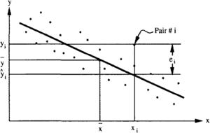
| − | [[File:Correlation-and-regression-analysis fig1.png|thumb|{{figure number|1}}Linear regression of x-on-y. Note the negative slope corresponding to a negative correlation. The regression line is determined so as to minimize the sum of squared deviations: <math>\sum_i{e_i^2}</math>]] | + | [[File:Correlation-and-regression-analysis fig1.png|300px|thumb|{{figure number|1}}Linear regression of x-on-y. Note the negative slope corresponding to a negative correlation. The regression line is determined so as to minimize the sum of squared deviations: <math>\sum_i{e_i^2}</math>]] |
Correlation analysis, and its cousin, regression analysis, are well-known statistical approaches used in the study of relationships among multiple physical properties. The investigation of [[permeability]]-[[porosity]] relationships is a typical example of the use of correlation in geology. | Correlation analysis, and its cousin, regression analysis, are well-known statistical approaches used in the study of relationships among multiple physical properties. The investigation of [[permeability]]-[[porosity]] relationships is a typical example of the use of correlation in geology. | ||
Revision as of 21:40, 20 May 2014
| Development Geology Reference Manual | |

| |
| Series | Methods in Exploration |
|---|---|
| Part | Geological methods |
| Chapter | Correlation and regression analysis |
| Author | T. C. Coburn |
| Link | Web page |
| PDF file (requires access) | |
Correlation analysis, and its cousin, regression analysis, are well-known statistical approaches used in the study of relationships among multiple physical properties. The investigation of permeability-porosity relationships is a typical example of the use of correlation in geology.
The term correlation most often refers to the linear association between two quantities or variables, that is, the tendency for one variable, x, to increase or decrease as the other, y, increases or decreases, in a straight-line trend or relationship.[1] [2] The correlation coefficient (also called the Pearson correlation coefficient), r, is a dimensionless numerical index of the strength of that relationship. The sample value of r, which can range from -1 to +1, is computed using the following formula:
where the summation is made over the n sample values available and where
- = ith observation of the first variable
- = corresponding ith observation of the second variable
- = corresponding sample (arithmetic) means
Many useful types of correlation other than simple linear correlation exist. Correlation based on the ranks (numerical ordering) of measurements of two variables is an important alternative for simple linear correlation when the number of samples is small and/or the joint distribution of the two variables is not simple. Multiple correlation and partial correlation are useful when studying relationships involving more than two variables. Cross correlation and autocorrelation are important to the analysis of repeated patterns observed in time and space, such as depth-related data recorded from geological stratigraphic sequences. Autocorrelation can also be used to measure the degree of similarity among porosity values measured at different locations.
Whereas correlation describes the linear association among variables, regression involves the prediction of one quantity from the others. Regression analysis is that broad class of statistics and statistical methods that comprises line, curve, and surface fitting, as well as other kinds of prediction and modeling techniques.
The simplest type of regression analysis involves fitting a straight line between two variables (Figure 1). In this case, one of the quantities is called the independent or predictor variable (usually denoted x), while the other is called the dependent or predicted variable (usually denoted y). This approach is often referred to as simple linear regression, or y-on-x regression. It leads to the development of an empirical straight-line relationship between the two variables and has the following form:
where
- a = slope
- b = y-intercept in an (x, y) coordinate system
One feature of this line is that it always passes through the centroid of the data () defined by the two arithmetic averages. The formulas for the parameters a and b are
- , and
There are two primary statistical applications for the regression line. It can be used as a sample-based estimate of an underlying linear functional relationship among the quantities of interest, or it can be employed as a predictive tool. To use the regression line for prediction, which is the most common usage in geology, simply substitute various values of x into the equation y = ax + b and solve for the corresponding predicted values of y.
By substituting the original x-values into the equation, it is possible to derive a measure of "goodness of fit" for the line. For every original x-value, a predicted value of y can be computed that differs from the corresponding original y-value by a certain amount. This difference, y - y, is called the residual e (in the y-direction), or deviation from the regression line. Two consequences of the least squares approach for the determination of the parameters a and b are that the sum of these residuals is zero and the sum of their squared values is as small as possible.
The sum of squares of the residuals is the basis for two measures of goodness of fit: the error variance s2 and the multiple correlation coefficient (also called the coefficient of determination). These two measures are given by the
following formulas:
where n is the number of (x, y) pairs.
The error variance s2 measures the scatter in the data about the regression line. The square of the sample correlation coefficient, R2, takes values from 0 to 1 and can be interpreted as the fraction of the variation in the data explained by the regression line. The line is said to be a good fit of the data if s2 is small and R2 is simultaneously large.
Some important extensions of two-variable linear regression analysis of particular interest to geologists include the following:
- Fitting through the origin, or forcing the regression line through any fixed point
- Regression in reverse, which consists of rewriting the regression of y-on-x as
- Modeling nonlinear relationships, such as
Various other functions of the x variable can be included in the previous relationship, such as polynomials and logarithms. Again, the regression parameters are determined so as to minimize the corresponding error variance.
Multiple and multivariate regression
The most important extension of the two-variable case is to situations involving more than two variables. When there is still one dependent variable but many predictor variables, the fitting technique is called multiple linear regression. When there are also more than one dependent variable, the approach is called multivariate regression (see Multivariate data analysis). The methods of simple bivariate regression extend directly to these multivariate situations. A typical geological application of multiple regression is the prediction of fold thickness from various geometric attributes, as given by the following equation:
Polynomial regression, sometimes referred to as curve fitting, is a special type of multiple regression frequently used in the earth sciences to model nonlinear relationships. Spline fitting is another type of nonlinear curve fitting. A close relative to polynomial curve fitting is surface fitting, which has one or more spatial components as predictor variables.
The fitting of surfaces by least squares is an important component in most automated contouring software packages and is commonly used in computer generation of geological maps. Trend surface analysis, another mapping technique, is also based on the principles of least-squares fitting. Finally, some of the more specialized geostatistical techniques, such as kriging, are likewise rooted in the basic principles of least squares and multiple regression.


