Faults: structural geology
| Oil Field Production Geology | |

| |
| Series | Memoir |
|---|---|
| Chapter | Structural geology: faults |
| Author | Mike Shepherd |
| Link | Web page |
| PDF file (requires access) | |
| Store | AAPG Store |
In structurally simple fields, the main control on production behavior is the distribution of lithofacies. In structurally complex fields, faults and fractures provide major elements influencing production performance. This article discusses the data used to establish the presence of faults and how faults are mapped for reservoir models. The reservoir structure can be analyzed at two different scales: the seismic scale and the well scale. The interpretation of faults and structure at the seismic scale is made by the seismic interpreter whereas the production geologist analyzes the structures from core and log data. Having established a fault framework for a field, it is important to know whether or not fluid flow communication occurs across the faults. Techniques are available to predict the likelihood of this. Sometimes sealing faults break down and open up to flow after a field has been producing for a few years. This reflects the change in the stress state of the reservoir as a result of pressure depletion.

Seismic interpretation of faults
The seismic data set is interpreted primarily using vertical time sections. These are displays that show a series of vertical seismic traces displayed side by side (Figure 1). The peaks or the troughs are filled in with black shading or color. Continuous reflections stand out as an overlapping array of peaks or troughs. These create patterns on a seismic section that give a representation of the geological structure in the subsurface. The seismic interpreter will look for discontinuities in the seismic reflections likely to represent faulting. Various techniques can help in picking faults. The interpretation can be cross checked against attribute maps showing changes in seismic dip (magnitude of the time gradient), azimuth (direction of maximum dip), or abrupt changes in amplitude.[2] [3] Another method is to use semblance data to detect edges in the data (see Lithofacies maps).
Structural core logging
Structural features such as fault zones and fractures are commonly seen in cores. Structural core logging may be required if there is a high density of such features or where knowledge of the detailed fault or fracture pattern is important for reservoir development.
Core goniometry is a method for graphically depicting the structure in the core. The whole core is wrapped around with acetate film, and the structures and main bedding planes in the core are traced directly with felt tip marker pens. The unrolled film shows a 360° depiction of the structure comparable to the display shown by borehole image logs. Commercial rigs are also available, which take 360° photographs of the core for the same purpose.
Having established the structures in the core, it is important to know how they were originally oriented within the reservoir. Dipmeter data, scribed core, and paleomagnetic data have all been used to work out the spatial orientation of the core.[4] [5]
Structural core logging provides a variety of useful information for the reservoir model. For example,
- the width of fault damage zones
- the orientation of the faults can be established and tied to the seismic interpretation
- the density and orientation of open fractures
- the composition and microstructure of material in the fault zone
Fault detection methods
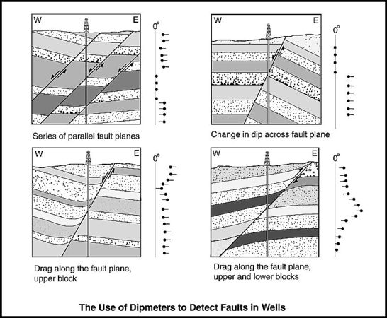
Figure 2 Dipmeter or image data can be used to pick likely fault planes in wells. Changes in dip amplitude or azimuth can indicate that a fault is present. Drag patterns may also be seen on the dip data above and below the fault intersection in a well (from Schlumberger[6]). Courtesy of Schlumberger.
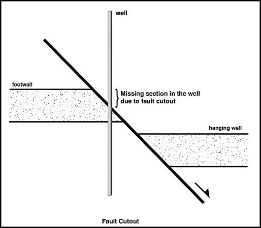
Figure 3 The stratigraphy in a well penetrating a normal fault will be incomplete due to fault cutout.
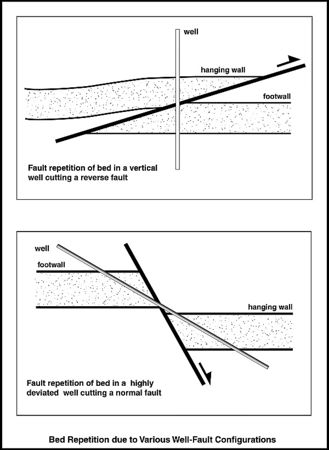
Figure 4 Repeated sections can be seen in a vertical well drilled through a reverse fault or with a highly deviated well penetrating a normal fault.


Dipmeter or borehole image data can be used to establish if and where any faults cut a well.[7] [8] [9] [10] A sharp change in dip amplitude or azimuth on a dipmeter log can indicate that a fault is present. Drag patterns may also be seen on the dip data above and below the fault intersection in the well (Figure 2).
An anomalously thin reservoir section, perhaps in conjunction with the absence of a reasonably persistent marker horizon, may be caused by a normal fault cutting out part of the stratigraphic section in a well (Figure 3). The thickness of missing section can be estimated by comparison to nearby wells with unfaulted sections.
A fault-repeated section is sometimes seen in a well (Figure 4). Near-vertical or gently dipping wells cutting reverse faults will show a repeated pattern. A repeat section can also occur where a highly deviated well cuts through a normal fault at a shallower angle than the dip of the fault plane (Figure 4).[11]
Well tests and faults

One method for locating faults is to check the results of reservoir engineering pressure transient analyses of well tests. The basis for these tests is that a production well, while it is flowing, will draw down the pressure for a considerable distance out into the surrounding reservoir. If the well is shut in and production is stopped, the pressure will build up as a result of the radial inflow of fluid toward the pressure sink in the immediate vicinity of the borehole. If a sealing fault or a feature likely to disrupt horizontal fluid inflow is present within the drainage radius of the well, then this can often be detected. The fault will disrupt the rate of pressure build-up once the catchment area for inflow of fluid increases outward with time and comes in contact with the fault plane (Figure 5). Analytical methods are available to make a rough estimate of how far away the fault is from the wellbore.
Care has to be taken that a feature such as a sand pinch-out or channel margin is not mistaken for a fault. It is a useful exercise for the reservoir engineer to have a working session with the seismic interpreter in order to compare test data for all the wells in the field with the interpreted fault pattern. An example of this is given by Marquez et al.[12] for the LL-04 reservoir in the Tia Juana field, Venezuela. An integrated reservoir characterization study was made to identify reserve growth opportunities. Part of this study involved cross checking the seismic interpretation of faults with evidence of compartmentalization from engineering data. In places where inferred reservoir compartments and faults did not coincide, the seismic interpretation was rechecked to see if a fault had been missed. If no fault could be located, the geologists then investigated the possibility that stratigraphic pinch-outs could be the cause of compartmentalization.
Mapping faults

Structure maps show the contoured depth surface and a representation of any faults cutting the surface. The faults are drawn as fault polygons marking the hanging wall and footwall fault cuts for the interpreted surface. The hanging wall is the rock volume above the fault plane, and the footwall is the rock volume that lies beneath it (Figure 3, Figure 4, Figure 6).
Faults on structure maps should be checked for consistency. The fault polygons represent the length of the fault that can be picked from seismic data. Where the fault throw is less than the seismic resolution, the fault will not be mapped by the interpreter. The limits of the seismically mapped faults will therefore not represent the actual fault tips in the subsurface, the points at either end of the real fault where the fault displacement is zero. Estimates can be made of the extent of the actual fault tips for a seismically mapped fault. The ideal normal fault trace will have an elliptical shape with the maximum displacement in the center of the fault, decreasing gradually to zero at the fault tips.[14] If a linear length-to-displacement ratio is assumed, it is possible to use this geometry to extend the seismic fault traces to a feasible location of the fault tips in the subsurface.[15]
If the structure is computer mapped, the contours interpolated by the mapping algorithm around faults can sometimes be rather untidy. It is not unusual for a computer map to show spurious fault reversal along the length of the fault. Thus, it is important to check and edit the contour maps by hand where this has happened.

Fault validation
Computer methods are available for validating the consistency of a reservoir fault framework. The most sophisticated of these will allow the geologist to examine the faulted model in 3-D and move the various fault blocks interactively back to the prefaulted undeformed state.[17] If this can be achieved without any gaps appearing, then the fault model is valid in a geometric sense. However, if large gaps cannot be removed, then there are serious problems with the structural interpretation. Sometimes it can take several attempts at making a fault interpretation before a validated fault model is obtained.
Zamora Valcarce et al.[16] used fault restoration to validate the El Porton field structure in Argentina prior to building a 3-D model of the field. The model was to be built to help plan the trajectories of new development wells. The idea behind validating the structural model was to give extra confidence that a planned well could be expected to intersect with the intended reservoir target given the structural complexities of the reservoir (Figure 7).

Fault restoration can also give insights into the structural history of an oil field. By determining the timing for episodes of faulting, uplift, and erosion, insights can be gained that allow the structural controls on reservoir development to be understood.
Fault geometries, linked faults, and relay ramps
What appears to be a simple large fault on seismic data may be more complex than it looks. The imaged fault may in reality comprise several closely spaced, overlapping faults, but because the seismic data cannot resolve the detail of the fault zone, it is shown as a single fault trace. These fault zones comprise linked fault segments with relay ramps in the overlapping areas between them (Figure 8).[18] [19]
It can be important to map relay ramps, as they can potentially provide pathways for fluid flow across a fault zone.[3] [20] Identification of relay ramps can be difficult in practice as the gap between overlapping faults are small (e.g., tens of meters) and difficult to resolve. However, there are ways in which relay ramps can be recognized, despite the limits of seismic resolution:
- Areas where fault traces show kinks on maps are commonly an expression of unresolved relay ramps.[21]
- Relay ramps may correspond to displacement minima along long faults.[19]
- Some of the longer faults may show anomalous length to displacement ratios. This can indicate that a relay ramp has been overlooked.[22]
Fault damage zone
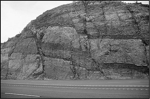
Figure 9 Fault damage zone from Moab, Utah. The outcrop is about 15 m (49 ft) high (photo courtesy of Angus MacLellan).
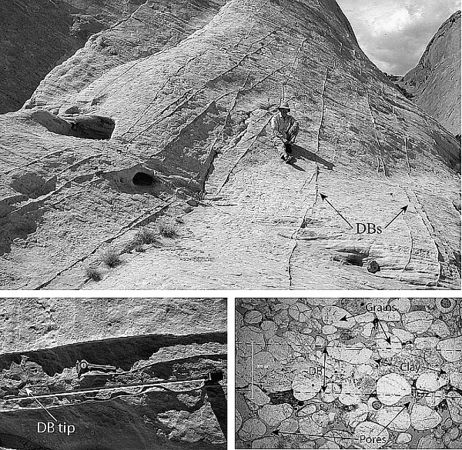
Figure 10 Deformation bands in the Aztec Sandstone, Valley of Fire, Nevada. Increased compaction compared to the undeformed rock causes the deformation bands to be more resistant to weathering and to stand out as ridges. Individual bands are approximately planar, showing distinct tips even where they are closely spaced (bottom left photo). Porosity loss resulting from granular rearrangement and clay accumulation in the bands results in lowered permeability (bottom right photo). DB = deformation band (from Sternlof et al.[23]).


A large number of fractures, microfaults, and deformation bands can be found in a zone (up to 100 m [328 ft] or more wide) on either side of major fault planes.[24] [25] [26] These damage zones can be observed in outcrops and in cores from wells near large faults (Figure 9).
Clean, porous sandstones respond to localized strain by forming deformation bands (Figure 10). These are tabular zones where the grains are reorganized by grain sliding, rotation, and commonly fracturing in response to deformation processes including dilation, shearing, and compaction.[27] Deformation bands are frequently sheared with shear offsets on a millimeter to centimeter scale. By comparison to open fractures, which tend to enhance permeability, deformation bands have a much reduced permeability compared to the undeformed host sandstone.[28] Given that a damage zone can contain hundreds of deformation bands, then it is clear that even sand-sand contact faults with damage zones can have significantly reduced permeability across them.
Damage zones in impure sandstones (those with 15–40% clay) contain phyllosilicate-framework fault rocks. These are anastomozing zones where the rock has been disaggregated and the clays have been mixed in with the framework grains to produce a more homogenous mixture of clays than is present in the undeformed host rock. Faults affecting clay-rich sandstones with more than 40% clay content form clay smears.[29]
The intensity of damage decreases away from the fault with the width of the damage zone roughly proportional to the throw of the fault.[30] [31] Field work on faulting in the Navajo Sandstone of Utah found that the summed width of the damage zones on either side of the fault core is approximately 2.5 times the total fault throw.[32] Note that this observation is case specific for this locality. Large and rapid variations in damage zone thickness occur along many faults, and any estimate attempting to systematically relate damage zone thickness to fault throw is liable to a significant uncertainty as a result.[33]
A study on the Big Hole Fault in Utah based on core data showed a significant permeability reduction within the damage zone.[34] Probe permeameter measurements of permeability range from more than 2000 md in the undeformed host sandstone to less than 0.1 md in fault-damaged rocks near the fault. Whole-core tests showed that the permeability of individual deformation bands vary between 0.9 and 1.3 md. The transverse permeability modeled over 5–10-m (16–32-ft)-length scales across the fault zone was estimated as 30–40 md. This is approximately 1–4% of the permeability for the undeformed host rock.
The general consensus in the industry is that damage zones around faults probably baffle flow across them rather than acting as barriers to fluid movement.[23] [33] The exception may be in deep reservoirs with high reservoir temperatures (more than 120°C). Here, accelerated quartz cementation at high temperature can decrease the pore throat diameters in the deformation bands to the extent that they become 100% water wet through capillary action. They thus become effective barriers to oil flow.[35]
Because of the abundance of low-permeability baffles and poorly connected volumes, production wells drilled in fault damage zones can significantly underperform. For example, wells drilled in fault-damaged zones in the North La Barge Shallow Unit of Wyoming are the poorest producers in the field.[36] It is generally not a good idea to plan a new well trajectory too close to a large fault because of this.
Faults and fluid flow
Faults can have a significant impact on the fluid flow patterns within a reservoir. They can juxtapose one reservoir interval with another creating the potential for cross flow between the units. It is pragmatic to assume that all sand to sand juxtapositions allow fluid transfer across faults unless proven otherwise.[37] Alternatively, juxtaposition of reservoir with nonreservoir rocks can cause the trapping of hydrocarbons against the fault. Deformation and cementation within the fault zone itself can create a zone of zero or very low permeability, which can cause the fault plane to act as a barrier to fluid flow. In some instances, fractures in the fault zone itself can act as conduits for fluid flow.

Allan diagrams
Allan diagrams or fault juxtaposition diagrams show the reservoir stratigraphy of both the hanging wall and footwall locations superimposed on the fault plane.[38] [39] At a glance, the juxtaposition relationships of the various reservoir units across the fault can be seen (Figure 11). Allan diagrams are useful for the production geologist but are subject to the uncertainty in the input data used. The magnitude of vertical fault displacement estimated from seismic data is prone to error. Additionally, where fault drag is present but not picked up on seismic data, the vertical fault displacement can be overestimated. Complex fault zone architecture can also create large uncertainties in establishing fault juxtaposition relationships.[40]
Fault seal
Estimates can be made using Allan diagrams as to the probability that a fault will seal within a reservoir. In the first instance, fault seal can result from the juxtaposition of reservoir with nonreservoir rock. However, experience from many petroleum provinces has shown that faults can seal even where reservoir quality sand bodies are juxtaposed across a fault. The most common mechanism for sealing results from the incorporation of fine grained or dense material into the fault plane. Five different processes may cause this:[41] [29]
- Clay smear: Faults in clay-rich sediments are believed to form clay smears by the shearing of mudstone beds into the fault zone.[42] [43]
- Cataclasis (shale gouge): Fault movement affecting clean sandstones will cause grain crushing and the breakage of rock in the fault plane, which will form a fault gouge.[44]
- Diagenesis or cementation: Fine grained fault rock and associated open fractures in fault zones can be prone to cementation. Fluids migrating up the fault zone can cause the mineralization of the host rock. It is a common observation to find carbonate-cemented intervals in wells drilled close to faults, whereas wells drilled farther away from the faults do not contain carbonate cements (e.g., Reynolds et al.[45]). This is an indication that the fault zones have acted as the locus for the fluids causing carbonate cementation.
- Pore volume collapse: Ductile deformation during fault movement can cause poorly sorted sediments to mix and homogenize with a resultant decrease in porosity.
- Grain contact dissolution: Fault zones can act as planes for intergranular grain contact dissolution and subsequent recementation of the dissolved material. This can be an important mechanism for fault sealing in carbonate rocks.[46]
When investigating fault seal, it is important to look at any faults in the core to determine which type of sealing mechanism may be present.
Fault sealing characteristics
Fine grained fault rock will have a higher capillary entry pressure compared to the undeformed host rock. Brown[47] described how the seal behavior of water-wet fault fill defines three potential zones within a fault.
- A fault can seal because the petroleum phase has insufficient buoyancy pressure to invade and displace water from the fine grained material within the fault rock; this has been termed membrane sealing.[48]
- Higher within the petroleum column, the buoyancy pressure can increase to the point at which the oil or gas can invade the fault rock and thus leak through it. However, the fault rock will have a very low permeability, and the rate of leakage can be trivial, even over geological time.[49] The fault can then be considered to be effectively lsquosealingrsquo by hydraulic resistance.[48]
- Where an exceptionally thick petroleum column exists, even low-permeability fault rocks can leak at significant rates. This is the zone of fault fill seal failure.
Fault seal prediction
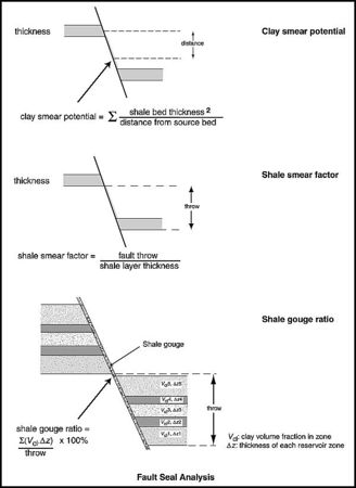
Figure 12 Fault seal analysis involves numerical methods of predicting the likelihood of fault seal (from Yielding et al.[50]).
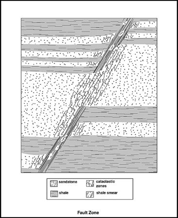
Figure 13 Schematic illustration showing the character of fault zones in siliciclastic strata based on outcrop and core observations from onshore and offshore Trinidad (from Gibson[51]).


Where sealing faults are a key element controlling the fluid flow in a reservoir, they should be characterized for reservoir description and modeling.[52] Much of the research to date has come about because of the particular importance of understanding fault behavior in deltaic reservoirs. In deltas deposited over thick and unstable mobile shale intervals, synsedimentary faults are a major element controlling reservoir continuity and size. The faults cut relatively unlithified sediments where the potential for clay smear along the fault planes is high and potentially predictable.
Algorithms are available for predicting the clay smear and shale gouge sealing potential of a fault. The basis for these algorithms is that the chances for clay smear to cause fault seal is controlled by the number and thickness of the shale beds displaced past a particular point on the fault. The thickness of the clay smear within the fault plane will decrease with distance from the source beds and with increasing throw of the fault.[50] The method involves taking the sand and shale distribution from a well close to the fault as a template for making the fault seal analysis.
The clay smear potential is calculated for a particular point on the fault plane as a function of the distance of that point from a shale bed acting as the source for the clay smear and the shale bed thickness[53] [54] (Figure 12).
The shale smear factor (SSF) is dependent on the shale bed thickness and the fault throw but not on the smear distance (Lindsay et al., 1993) (Figure 12). Smaller values of the SSF correspond to a more continuous development of smear on the fault plane. A large fault is likely to seal where the SSF is equal to or less than 4.[55]
The shale gouge ratio works on the assumption that the sealing capacity is related directly to the percentage of shale beds or clay material within the slipped interval.[50] The shale gouge ratio is the proportion of the sealing lithology in the rock interval that has slipped past a given point on the fault (Figure 12). To calculate the shale gouge ratio, the proportion of shale and clay in a window equivalent to the throw is measured.
The prediction of fault seal is based on the assumption that if there is enough shale in the section undergoing faulting, then sealing is likely. There is often a continuous shale gouge or shale smear along fault planes where there is sufficient mudstone material available to be incorporated.[44] [56] Nevertheless, a number of field studies show that fault zones can have a significant degree of complexity and variation in deformation style along their lengths.[57] [58] For example, Foxford et al.[56] examined good exposures of the Moab fault in Utah. They found that the structure and content of the fault zone was so variable that it was impossible to predict the nature of the fault zone over even a 10-m (33-ft) distance. Doughty[59] found that the clay smear along the Calabacillas fault in New Mexico showed numerous gaps particularly where minor faults within the fault zone complex cut out the shale smear associated with the major slip plane. The implication of these field studies is that fault seal can be predicted but is subject to chance factors affecting the reliability of the prediction. Because of this, any fault seal prediction should be calibrated against actual evidence that fault compartmentalization is present. Yielding et al.[60] made a fault seal analysis for the Gullfaks field in the Norwegian North Sea. Areas of higher shale gouge ratios (>20%) were more likely to seal on the basis of pressure history and chemical tracer movement between wells.
Gibson[51] provided a case history for fault seal analysis from the Columbus Basin, offshore Trinidad. Oil and gas fields occur in upper Miocene to Pleistocene deltaic sandstones of the Columbus Basin, located offshore to the southeast of the island of Trinidad. Numerous small faults dissect these reservoirs, and fault seal appears to be a critical feature controlling the size of these petroleum pools. Allan diagrams show that juxtaposition sealing is insufficient to explain the fault control on fluid contacts.
The sediments that form the reservoirs offshore are also exposed onshore along the east coast of Trinidad. Outcrops onshore and cores offshore provide control on the nature of the fault rock. In these outcrops, shale smears are found where shale beds have been displaced along the fault. The shale smears range in thickness from millimeter- to centimeter-thick shale partings to complex zones up to several meters thick (Figure 13).
Offshore, hydrocarbon columns up to 200 m (656 ft) thick are found within compartments interpreted as being sealed by clay smears along faults. The general observation is that the blanket of clay smear along faults only appears to be continuous and effective where the shale content of the displaced section exceeds 25%. The shale smear factor was estimated for faults from two of the fields in the basin. SSF values of between 1 and 4 were found for faults with throws more than 150 m (492 ft) that sealed the longest hydrocarbon columns. It was concluded that faults in this area could be modeled as sealing along their length provided the SSF did not exceed a value of 4.
Subseismic faults
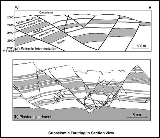
Figure 14 Comparison between (a) depth-converted seismic interpretation from the Gullfaks field, Norwegian North Sea, and (b) a plaster model deformed by plane strain extension. The plaster model shows that many small-scale faults are expected to exist in the Gullfaks structure but are below seismic resolution (from Fossen and Hesthammer[61]). Reprinted with permission from the Geological Society of London.
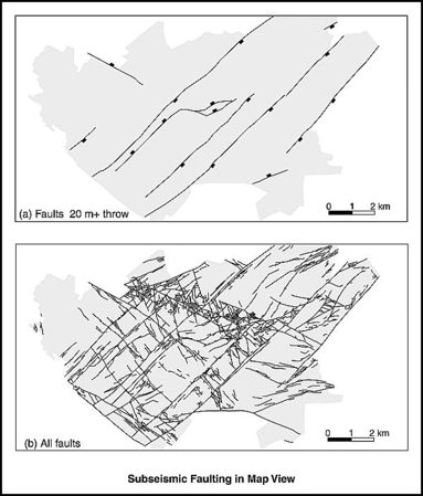
Figure 15 Fault maps of the East Pennine coalfield, United Kingdom. In map (a), only faults with throws of 20 m (64 ft) or more are shown. These are equivalent to faults that are detectable by seismic surveys at reservoir depths. In map (b), every mapped fault is shown, with fault throws of between 10 cm (4 in.) and 180 m (590 ft) (from Watterson et al.[62]). Reprinted with permission from the Journal of Structural Geology.


Only the faults that the geophysicist can pick from seismic data will be mapped, that is, those faults with vertical displacements down to the limit of seismic resolution. As mentioned in Data: sources, this can be about 20–40 m for reservoirs at moderate depths. However, a significant number of subseismic faults will probably be present with vertical displacements less than this (Figure 14, Figure 15). Thus, the true degree of the structural complexity of a reservoir will be underrepresented.
It is possible to input subseismic faults into a reservoir model using stochastic methods.[63] [64] In summary, this is a computerized procedure for randomly inserting shapes representing geological features into a 3-D model while still honoring predefined rules and statistics controlling the global distribution of the data.
The first part of the method involves making an estimate of the number of subseismic faults by extrapolating from statistics on the length versus frequency of known seismic faults into the subseismic region. Fractal analysis has been used on the assumption that fault-size populations approximate to fractal distributions.[65] Statistics are also compiled on fault orientations, length to throw ratios, and fault densities per square kilometer. A further step is to determine those areas of the field where subseismic faults are more likely to be present than elsewhere. One method is to predict the paleostrain regime of the reservoir at the time of faulting.[66] On this basis, a model will be made, which will include both the seismic and subseismic faults. Fault seal analysis can be applied to the subseismic faults in the model to determine whether they are sealing or not.
General experience with inserting subseismic faults into simulation models is that they will influence the flow behavior.[67] [68] [69] The critical feature seems to be whether the faults are sealing or not. Sealing faults can create an open framework of short baffles, which helps to improve sweep. The baffles increase the tortuosity of the flood front and delay water breakthrough. A large number of sealing subseismic faults in a reservoir will, on the other hand, create numerous dead ends, which will reduce the sweep efficiency of a waterflood. Nonsealing subseismic faults form cross-fault juxtapositions, which can improve vertical connectivity and enhance sweep.

Growth faults
Growth faults are faults that were active at the same time as the sediments were being deposited (Figure 16). Many show a listric geometry with the fault soling out into shale horizons. They are common in areas with thick delta sequences. Growth faults can be recognized because sediments thicken into the hanging wall of a growth fault and the throw of the fault increases with depth. All the individual reservoir units may thicken up across a mapped growth fault. Alternatively, growth can be taken up by additional layers filling the accommodation space in the hanging wall.[71]
Faults as flow conduits
It is known that faults can conduct flow along the fault plane. Brittle rocks such as carbonates are more likely to contain conductive faults by comparison to shallow buried siliciclastic sediments, for example.
Specific examples of faults acting as fluid conduits have been described. Production wells located near faults showed rapid water breakthrough in the Fateh field, offshore Dubai. Well tests, production logs, radioactive tracer surveys, and interference tests indicate that aquifer influx is occurring along conductive faults within the reservoir.[72] A campaign of horizontal drilling in the Prudhoe Bay field in Alaska showed that between 10 and 20% of the faults intersected by the wells were conductive to flow. These caused early water or gas production as a result of fault intersection with the water leg or the gas cap.[73] Production, pressure, and production log data indicated that water flowing up faults had resulted in rapid water breakthrough in the crestal area of the Khafji field in the Arabian Gulf.[74]
Stress changes in reservoirs
In stress-sensitive reservoirs, fractures may dilate during injection and close during drawdown. These effects are most pronounced in low-permeability, overpressured, and naturally fractured reservoirs.[75] Pressure depletion as a result of production will change the stress state of a reservoir (e.g., Hillis[76]).
From a mechanical aspect, sandstone reservoirs are porous structures that form a load-bearing framework supporting the weight of the overburden. Reservoir depletion increases the effective stress on the grain framework; this is the difference between the total stress acting on all sides of the rock and the pore fluid pressure. The effective stress is applied at the grain to grain contacts. This leads to elastic deformation of the rock (recoverable on depletion reversal) and, with increasing stress, inelastic deformation. Inelastic deformation mechanisms include microcrack growth and closure, cement breakage, grain rotation, and sliding as well as deformation in clay, mica, and diagenetically altered feldspar grains.[77] [78] [79] [80] These mechanisms result in the compaction of the rock and a reduction in the porosity. Because the reservoir remains physically connected to the rock surrounding it, the overburden and underburden will also deform in response to reservoir depletion.
Compaction can lead to the reactivation of normal faults.[81] [82] In the Valhall and Ekofisk fields, offshore Norway, faults that were initially located in the crest of the field's anticlinal structure are thought to have spread out to the flanks as a result of reactivation induced by depletion and compaction of the Chalk reservoir. Casing failures have been attributed to shear along these spreading faults.[83] Small earthquakes can be common around some producing oil and gas fields.[84]
It is common to find that faults that were sealing over geological time in a reservoir start to leak after a few years of production. This may be noticed where a production anomaly occurs, such as newly drilled attic oil wells showing swept zones; a sudden, unexpected rapid rise in water or hydrocarbon production from production wells drilled close to faults; or an inexplicable source of pressure support appearing in the mid life of a producing well. In one example from the Endicott field in Alaska, a major sealing fault within the reservoir was known to act as a pressure barrier from early production data. Later on, it was established that radioactive tracer had crossed the fault from an injection well to a production well, and this indicated that the fault seal had broken down with production.[85]
Dincau[86] analyzed fault breakdown with production in the South Marsh Island 66 field, offshore Louisiana. The faults most likely to break down were those with limited predicted shale gouge and where the reservoir unit was fault juxtaposed against itself. Faults with an extensive predicted shale gouge and where they juxtapose one reservoir unit with a different unit were more likely to hold a pressure differential.
Examples of fault breakdown are often mentioned as a side issue in technical papers dealing with other aspects of field production. These include the Iagufu-Hedinia area of Papua New Guinea,[87] the Tia Juana field in Venezuela,[88] and the Veslefrikk field, offshore Norway.[89] Fault breakdown is often attributed to the breaching of the capillary seal of the fault rock as a result of large differences in pressure across the fault. It is also possible that in some instances, fault breakdown is the result of fault reactivation induced by differential compaction between adjacent fault compartments, one significantly more depleted than the other. It is possible that the phenomena could be more common in depleting fields than is generally appreciated.
See also
References
- ↑ Dominguez, R., 2007, Structural evolution of the Penguins cluster, UK northern North Sea, in S. J. Jolley, D. Barr, J. J. Walsh, and R. J. Knipe, eds., Structurally complex reservoirs: Geological Society (London) Special Publication 292, p. 25–48.
- ↑ Dalley, R. M., E. E. A. Gevers, G. M. Stampli, D. J. Davies, C. N. Gastaldi, P. R. Ruijetnberg, and G. J. D. Vermeer, 1989, Dip and azimuth displays for 3-D seismic interpretation: First Break, v. 7, p. 86–95.
- ↑ 3.0 3.1 Hesthammer, J., and H. Fossen, 1997, Seismic attribute analysis in structural interpretation of the Gullfaks field, northern North Sea: Petroleum Geoscience, v. 3, no. 1, p. 13–26.
- ↑ Davison, I., and R. S. Haszeldine, 1984, Orienting conventional cores for geological purposes: A review of methods, Journal of Petroleum Geology, v. 7, no. 4, p. 461–466.
- ↑ Bleakly, D. C., 1992, Core orientation, in D. Morton-Thompson and A. M. Woods, eds., Development geology reference manual: AAPG Methods in Exploration Series 10, p. 122–124.
- ↑ Schlumberger, 1981, Dipmeter interpretation, volume 1—Fundamentals: New York, Schlumberger, 61 p.
- ↑ Bengtson, C. A., 1981, Statistical curvature analysis techniques for structural interpretation of dipmeter data: AAPG Bulletin, v. 65, no. 2, p. 312–332.
- ↑ Bengtson, C. A., 1982, Structural and stratigraphic uses of dip profiles in petroleum exploration, in M. T. Halbouty, ed., The deliberate search for the subtle trap: AAPG Memoir 32, 351 p.
- ↑ Goetz, J. F., 1992, Dipmeters, in D. Morton-Thompson and A. M. Woods, eds., Development geology reference manual: AAPG Methods in Exploration Series 10, p. 158–162.
- ↑ Adams, J. T., and C. Dart, 1998, The appearance of potential sealing faults on borehole images, in G. Jones, Q. J. Fisher, and R. J. Knipe, eds., Faulting, fault sealing and fluid flow in hydrocarbon reservoirs: Geological Society (London) Special Publication 147, p. 71–86.
- ↑ Mulvany, P. S., 1992, A model for classifying and interpreting logs of boreholes that intersect faults in stratified rocks: AAPG Bulletin, v. 76, no. 6, p. 895–903.
- ↑ Marquez, L. J., M. Gonzalez, S. Gamble, E. Gomez, M. A. Vivas, H. M. Bressler, L. S. Jones, S. M. Ali, and G. S. Forrest, 2001, Improved reservoir characterization of a mature field through an integrated multi-disciplinary approach, LL-04 reservoir, Tia Juana field, Venezuela: Presented at the Society of Petroleum Engineers Annual Technical Conference and Exhibition, September 30–October 3, New Orleans, Louisiana, SPE Paper 71355, 10 p.
- ↑ Gluyas, J. G., and J. R. Underhill, 2003, The Staffa field, Block 3/8b, UK North Sea, in J. G. Gluyas and H. M. Hichens, eds., United Kingdom oil and gas fields, commemorative millennium volume: Geological Society (London) Memoir 20, p. 327–333.
- ↑ Barnett, J. A. M., J. Mortimer, J. H. Rippon, J. J. Walsh, and J. Watterson, 1987, Displacement geometry in the volume containing a single normal fault: AAPG Bulletin, v. 71, no. 8, p. 925–937.
- ↑ Pickering, G., D. C. P. Peacock, D. J. Sanderson, and J. M. Bull, 1997, Modeling tip zones to predict the throw and length characteristics of faults: AAPG Bulletin, v. 81, no. 1, p. 82–89.
- ↑ 16.0 16.1 Zamora Valcarce, G., T. Zapata, A. Ansa, and G. Selva, 2006, Three-dimensional modeling and its application for development of the El Porton field, Argentina: AAPG Bulletin, v. 90, no. 3, p. 307–319.
- ↑ Williams, G. D., S. J. Kane, T. S. Buddin, and A. J. Richards, 1997, Restoration and balance of complex folded and faulted rock volumes: Tectonophysics, v. 273, no. 3–4, p. 203–218.
- ↑ 18.0 18.1 Peacock, D. C. P., and D. J. Sanderson, 1994, Geometry and displacement of relay ramps on normal fault systems: AAPG Bulletin, v. 78, no. 2, p. 147–165.
- ↑ 19.0 19.1 Needham, D. T., G. Yielding, and B. Freeman, 1996, Analysis of fault geometry and displacement patterns, in P. G. Buchanan and D. A. Nieuwland, eds., 1996, Modern developments in structural interpretation, validation and modelling: Geological Society Special Publication 99, p. 189–199.
- ↑ Rotevatn, A., H. Fossen, J. Hesthammer, T. E. Aas, and J. A. Howell, 2007, Are relay ramps conduits for fluid flow? Structural analysis of a relay ramp in Arches National Park, Utah, in L. Lonergan, R. Jolly, K. Rawnsley, and D. J. Sanderson, eds., Fractured reservoirs: Geological Society (London) Special Publication 270, p. 55–71.
- ↑ Fossen, H., T. S. Johansen, J. Hesthammer, and A. Rotevatn, 2005, Fault interaction in porous sandstone and implications for reservoir management, examples from southern Utah: AAPG Bulletin, v. 89, no. 12, p. 1593–1606.
- ↑ Willemse, E. J. M., D. D. Pollard, and A. Aydin, 1996, Three-dimensional analyses of slip distributions on normal fault arrays with consequences for fault scaling: Journal of Structural Geology, v. 18, no. 2–3, p. 295–309.
- ↑ 23.0 23.1 Sternlof, K. R., J. R. Chapin, D. D. Pollard, and L. J. Durlofsky, 2004, Permeability effects of deformation band arrays in sandstone: AAPG Bulletin, v. 88, no. 9, p. 1315–1329.
- ↑ Aydin, A., and A. M. Johnson, 1978, Development of faults as zones of deformation bands and as slip surfaces in sandstones: Pure and Applied Geophysics, v. 116, p. 931–942.
- ↑ Jamison, W. R., and D. W. Stearns, 1982, Tectonic deformation of Wingate Sandstone, Colorado National Monument: AAPG Bulletin, v. 66, no. 12, p. 2584–2608.
- ↑ Antonellini, M., and A. Aydin, 1995, Effects of faulting on fluid flow in porous sandstones: Geometry and spatial distribution: AAPG Bulletin, v. 79, no. 5, p. 642–670.
- ↑ Fossen, H., R. A. Schultz, Z. K. Shipton, and K. Mair, 2007, Deformation bands in sandstone: A review: Journal of the Geological Society (London), v. 164, p. 755–769.
- ↑ Antonellini, M., and A. Aydin, 1994, Effect of faulting on fluid flow in porous sandstones: Petrophysical properties: AAPG Bulletin, v. 78, no. 3, p. 355–377.
- ↑ 29.0 29.1 Fisher, Q. J., and R. J. Knipe, 1988, Fault sealing processes in siliciclastic sediments, in H. Jones, Q. J. Fisher, and R. J. Knipe, eds., Faulting, fault sealing and fluid flow in hydrocarbon reservoirs: Geological Society (London) Special Publication 147, p. 117–134. Cite error: Invalid
<ref>tag; name "Fisherandknipe_1998" defined multiple times with different content - ↑ Knott, S. D., 1994, Fault zone thickness versus displacement in the Permo-Triassic sandstones of NW England: Journal of the Geological Society, v. 151, p. 17–25.
- ↑ Knott, S. D., A. Beach, P. J. Brockbank, J. L. Brown, J. E. McCallum, and A. I. Welbon, 1996, Spatial and mechanical controls on normal fault populations: Journal of Structural Geology, v. 18, no. 2/3, p. 359–372.
- ↑ Shipton, Z. K., and P. A. Cowie, 2001, Damage zone development over micron to kilometer scales in high-porosity Navajo sandstone, Utah: Journal of Structural Geology, v. 23, p. 1825–1844.
- ↑ 33.0 33.1 Fossen, H., and A. Bale, 2007, Deformation bands and their influence on fluid flow: AAPG Bulletin, v. 91, no. 12, p. 1685–1700.
- ↑ Shipton, Z. K., J. P. Evans, K. R. Robeson, C. B. Forster, and S. Snelgrove, 2002, Structural heterogeneity and permeability in faulted eolian sandstone: Implications for subsurface modeling of faults: AAPG Bulletin, v. 86, no. 5, p. 863–883.
- ↑ Hesthammer, J., P. A. Bjorkum, and L. Watts, 2002, The effect of temperature on sealing capacity of faults in sandstone reservoirs: Examples from the Gullfaks and Gullfaks Sor fields, North Sea: AAPG Bulletin, v. 86, no. 10, p. 1733–1751.
- ↑ Miskimins, J. L., 2003, Analysis of hydrocarbons production in a critically-stressed reservoir: Presented at the Society of Petroleum Engineers Annual Technical Conference and Exhibition, October 5–8, Denver, Colorado, SPE Paper 84457, 8 p.
- ↑ James, W. R., L. H. Fairchild, G. P. Nakayama, S. J. Hippler, and P. J. Vrolijk, 2004, Fault-seal analysis using a stochastic multi-fault approach: AAPG Bulletin, v. 88, no. 7, p. 885–904.
- ↑ Allan, U. S., 1989, Model for hydrocarbon migration and entrapment within faulted structures: AAPG Bulletin, v. 73, no. 7, p. 803–811.
- ↑ Knipe, R. J., 1997, Juxtaposition and seal diagrams to help analyze fault seals in hydrocarbon reservoirs: AAPG Bulletin, v. 81, no. 2, p. 187–195.
- ↑ Hesthammer, J., and H. Fossen, 2000, Uncertainties associated with fault sealing analysis: Petroleum Geoscience, v. 6, p. 37–45.
- ↑ Mitra, S., 1988, Effects of deformation mechanisms on reservoir potential in central Appalachian overthrust belt: AAPG Bulletin, v. 72, no. 5, p. 536–554.
- ↑ Weber, K. J., L. J. Urai, W. F. Pilaar, F. Lehner, and R. G. Precious, 1978, The role of faults in hydrocarbon migration and trapping in Nigerian growth fault structures: 10th Annual Offshore Technology Conference Proceedings, v. 4, p. 2643–2653.
- ↑ Lehner, F. K., and F. K. Pilaar, 1997, The emplacement of clay smears in synsedimentary normal faults: Inferences and field observations near Frechen Germany, in P. Moller-Pederson and A. G. Koestler, eds., Hydrocarbon seals: Importance for exploration and production: Norwegian Petroleum Society Special Publication 7, p. 15–38.
- ↑ 44.0 44.1 Lindsay, N. G., F. C. Murphy, J. J. Walsh, and J. Watterson, 1993, Outcrop studies of shale smear on fault surfaces, in S. S. Flint and I. D. Bryant, eds., The geological modelling of hydrocarbon reservoirs and outcrop analogs: International Association of Sedimentologists Special Publication 15, p. 113–123.
- ↑ Reynolds, A. D., et al., 1998, Implications of outcrop geology for reservoirs in the Neogene productive series: Apsheron Peninsula, Azerbaijan: AAPG Bulletin, v. 82, no. 1, p. 25–29.
- ↑ Peacock, D. C. P., Q. J. Fisher, E. J. M. Willemse, and A. Aydin, 1998, The relationship between faults and pressure solution seams in carbonate rocks and the implications for fluid flow, in G. Jones, Q. J. Fisher, and R. J. Knipe, eds., Faulting and fluid flow in hydrocarbon reservoirs: Geological Society (London) Special Publication 147, p. 105–115.
- ↑ Brown, A., 2003, Capillary effects on fault-fill sealing: AAPG Bulletin, v. 87, no. 3, p. 381–395.
- ↑ 48.0 48.1 Watts, N. L., 1987, Theoretical aspects of cap-rock and fault seals for single and two phase columns: Marine and Petroleum Geology, v. 4, no. 4, p. 274–307.
- ↑ Heum, O. R., 1996, A fluid dynamic classification of hydrocarbon entrapment: Petroleum Geoscience, v. 2, no. 2, p. 145–158.
- ↑ 50.0 50.1 50.2 Yielding, G., B. Freeman, and D. T. Needham, 1997, Quantitative fault seal prediction: AAPG Bulletin, v. 81, no. 6, p. 897–917.
- ↑ 51.0 51.1 Gibson, R. G., 1994, Fault-zone seals in siliciclastic strata of the Columbus basin, offshore Trinidad: AAPG Bulletin, v. 78, no. 9, p. 1372–1385.
- ↑ Fisher, Q. J., and S. J. Jolley, 2007, Treatment of faults in production simulation models, in S. J. Jolley, D. Barr, J. J. Walsh, and R. J. Knipe, eds., Structurally complex reservoirs: Geological Society (London) Special Publication 292, p. 219–233.
- ↑ Bouvier, J. D., C. H. Kaars-Sijpesteijn, D. F. Kluesner, C. C. Onyejekwe, and R. C. Van der Pal, 1989, Three-dimensional seismic interpretation and fault sealing investigations, Nun River field, Nigeria: AAPG Bulletin, v. 73, p. 1397–1414.
- ↑ Fulljames, J. R., L. J. J. Zijerveld, and R. C. M. W. Fransen, 1997, Fault seal processes: Systematic analysis of fault seals over geological and production time scales, in P. Moller-Petersen and A. G. Koestler, eds., Hydrocarbon seals, importance for exploration and production: Norwegian Petroleum Society Special Publication 7, p. 51–79.
- ↑ Farseth, R. B., 2006, Shale smear along large faults: Continuity of smear and fault seal capacity: Journal of the Geological Society (London), v. 163, p. 741–751.
- ↑ 56.0 56.1 Foxford, K. A., J. J. Walsh, J. Watterson, I. R. Garden, S. C. Guscott, and S. D. Burley, 1998, Structure and content of the Moab fault zone, Utah, U.S.A., and its implications for fault seal prediction, in H. Jones, Q. J. Fisher, and R. J. Knipe, eds., Faulting, fault sealing and fluid flow in hydrocarbon reservoirs: Geological Society (London) Special Publication 147, p. 87–103.
- ↑ Childs, C., J. J. Walsh, and J. Watterson, 1997, Complexity in fault zones and its implications for fault seal prediction, in P. Moller-Pederson and A. G. Koestler, eds., Hydrocarbon seals: Importance for exploration and production: Norwegian Petroleum Society Special Publication 7, p. 61–72.
- ↑ James, D. M. D., C. Childs, J. Watterson, and J. J. Walsh, 1997, Discussion on a model for the structure and development of fault zones: Reply: Journal of the Geological Society (London), v. 154, no. 2, p. 366–368.
- ↑ Doughty, P. T., 2003, Clay smear seals and fault sealing potential of an exhumed growth fault, Rio Grande rift, New Mexico: AAPG Bulletin, v. 87, no. 3, p. 427–444.
- ↑ Yielding, G., J. A. Overland, and G. Byberg, 1999, Characterization of fault zones for reservoir modeling: An example from the Gullfaks field, northern North Sea: AAPG Bulletin, v. 83, no. 6, p. 925–951.
- ↑ Fossen, H., and J. Hesthammer, 1998, Structural geology of the Gullfaks field, northern North Sea, in M. P. Coward, H. Johnson, and T. S. Daltaban, eds., Structural geology in reservoir characterization: Geological Society Special Publication 127, p. 231–261.
- ↑ Watterson, J., J. J. Walsh, P. A. Gillespie, and S. Easton, 1996, Scaling systematics of fault sizes on a large-scale range fault map: Journal of Structural Geology, v. 18, no. 2/3, p. 199–214.
- ↑ Munthe, K. L., H. Omre, L. Holden, E. Damsleth, K. Heffer, T. S. Olsen, and J. Watterson, 1993, Subseismic faults in reservoir description and simulation, Presented at the Society of Petroleum Engineers Annual Technical Conference and Exhibition, October 3–6, Houston, Texas, SPE Paper 26500, 8 p.
- ↑ Hollund, K., P. Mostad, B. F. Nielsen, L. Holden, J. Gjerde, M. G. Contursi, A. J. McCann, C. Townsend, and E. Sverdrup, 2002, Havana—A fault modelling tool, in A. G. Koestler and R. Hunsdale, eds., Hydrocarbon seal quantification: Norwegian Petroleum Society Special Publication 11, p. 157–171.
- ↑ Gauthier, B. D. M., and S. D. Lake, 1993, Probabilistic modeling of faults below the limit of seismic resolution in Pelican field, North Sea, offshore United Kingdom: AAPG Bulletin, v. 77, no. 5, p. 761–777.
- ↑ Maerten, L., P. Gillespie, and J.-M. Daniel, 2006, Three-dimensional geomechanical modeling for constraint of subseismic fault simulation: AAPG Bulletin, v. 90, no. 9, p. 1337–1358.
- ↑ Damsleth, E., V. Sangolt, and G. Aamodt, 1998, Sub-seismic faults can seriously affect fluid flow in the Njord field off western Norway—A stochastic fault modeling case study: Presented at the 1998 Society of Petroleum Engineers Annual Technical Conference and Exhibition, September 27–30, 1998, New Orleans, SPE Paper 49024, 49 p.
- ↑ England, W. A., and C. Townsend, 1998, The effects of faulting on production from a shallow marine reservoir: Presented at the 1998 Society of Petroleum Engineers Annual Technical Conference and Exhibition, September 27–30, 1998, New Orleans, SPE Paper 49023, 16 p.
- ↑ Ottesen, S., C. Townsend, and K. M. Overland, 2005, Investigating the effect of varying fault geometry and transmissibility on recovery: Using a new workflow for structural uncertainty modeling in a clastic reservoir, in P. Boult and J. Kaldi, eds., Evaluating fault and cap rock seals: AAPG Hedberg Series 2, p. 125–136.
- ↑ Edwards, M. B., 1976, Growth faults in upper Triassic deltaic sediments, Svalbard: AAPG Bulletin, v. 60, no. 3, p. 341–355.
- ↑ Hodgetts, D., J. Imber, C. Childs, S. Flint, J. Howell, J. Kavanagh, P. Nell, and J. Walsh, 2001, Sequence-stratigraphic responses to shoreline-perpendicular growth faulting in shallow marine reservoirs of the Champion field, offshore Brunei Darussalam, South China Sea: AAPG Bulletin, v. 85, no. 3, p. 433–457.
- ↑ Trocchio, J. T., 1990, Investigation of Fateh Mishrif fluid-conductive faults: Journal of Petroleum Technology, v. 42, no. 8, SPE Paper 17992, p. 1038–1045.
- ↑ Pucknell, J. K., and W. H. Broman, 1994, An evaluation of Prudhoe Bay horizontal and high-angle wells after 5 years of production: Journal of Petroleum Technology, v. 46, no. 2, SPE Paper 26596, p. 150–156.
- ↑ Nishikiori, N., and Y. Hayashida, 1999, Investigation and modeling of complex water influx into the sandstone reservoir, Khafji oil field, Arabian Gulf: Presented at the Society of Petroleum Engineers Annual Technical Conference and Exhibition, October 3–6, Houston, Texas, SPE Paper 56428, 16 p.
- ↑ Lorenz, J. C., 1999, Stress-sensitive reservoirs: Journal of Petroleum Technology, SPE Paper 50977, v. 51, no. 1, p. 61–63.
- ↑ Hillis, R. R., 2001, Coupled changes in pore pressure and stress in oilfields and sedimentary basins: Petroleum Geoscience, v. 7, no. 4, p. 419–425.
- ↑ Bernabe, Y., D. T. Fryer, and R. M. Shively, 1994, Experimental observations of the elastic and inelastic behaviour of porous sandstones: Geophysical Journal International, v. 199, p. 403–418.
- ↑ Schutjens, P. M. T. M., T. L. Blanton, J. W. Martin, B. C. Lehr, and M. N. Baaijens, 1998, Depletion-induced compaction of an overpressured reservoir sandstone: Experimental approach: Society of Petroleum Engineers Paper 47277, 10 p.
- ↑ Schutjens, P. M. T. M., T. H. Hanssen, M. H. H. Hettema, J. Merour, P. de Bree, J. W. A. Coremans, and G. Helliesen, 2004, Compaction-induced porosity/permeability reduction in sandstone reservoirs: Data and model for elasticity-dominated deformation: Presented at the 2001 Society of Petroleum Engineers Annual Technical Conference and Exhibition, September 30–October 3, New Orleans, SPE Reservoir Evaluation and Engineering, SPE Paper 88441, v. 7, no. 3, p. 202–216.
- ↑ Wong, T.-F., and P. Baud, 1999, Mechanical compaction of porous sandstone: Oil and Gas Science and Technology Review, v. 54, p. 785–797.
- ↑ Teufel, L. W., D. W. Rhett, and H. E. Farrell, 1991, Effect of reservoir depletion and pore pressure drawdown on in situ stress and deformation in the Ekofisk field, North Sea, in J. C. Rogiers, ed., Rock mechanics as an multidisciplinary science: Rotterdam, Balkema, p. 63–72.
- ↑ Goulty, N. R., 2003, Reservoir stress path during depletion of Norwegian chalk oil fields: Petroleum Geoscience, v. 9, p. 233–241.
- ↑ Zoback, M. D., and J. C. Zinke, 2002, Production-induced normal faulting in the Valhall and Ekofisk oil fields: Pure and Applied Geophysics, v. 159, no. 1–3, p. 403–420.
- ↑ Segall, P., 1989, Earthquakes triggered by fluid extraction: Geology, v. 17, p. 942–946.
- ↑ Shaw, A., A. Reynolds, and E. Warren, 1996, Integrated description of a complex low net/gross sandstone reservoir: Upper subzones of the Endicott field, north slope of Alaska: Presented at the European 3-D Reservoir Modeling Conference, Society of Petroleum Engineers, April 16–17, Stavanger, Norway, SPE Paper 35496, 13 p.
- ↑ Dincau, A. R. 1998, Prediction and timing of production induced fault seal breakdown in the South Marsh Island 66 gas field: Gulf Coast Association of Geological Societies Transactions, v. 48, p. 21–32.
- ↑ Eisenberg, L. I., M. V. Langston, and R. E. Fitzmorris, 1994, Reservoir management in a hydrodynamic environment, Iagufu-Hedinia area, Southern Highlands, Papua New Guinea: Presented at the Society of Petroleum Engineers Asia Pacific Oil and Gas Conference, November 7–10, Melbourne, Australia, SPE Paper 28750, 17 p.
- ↑ Marquez, L. J., M. Gonzalez, S. Gamble, E. Gomez, M. A. Vivas, H. M. Bressler, L. S. Jones, S. M. Ali, and G. S. Forrest, 2001, Improved reservoir characterization of a mature field through an integrated multi-disciplinary approach, LL-04 reservoir, Tia Juana field, Venezuela: Presented at the Society of Petroleum Engineers Annual Technical Conference and Exhibition, September 30–October 3, New Orleans, Louisiana, SPE Paper 71355, 10 p.
- ↑ Pedersen, P., R. Hauge, and E. Berg, 1994, The Veslefrikk field, in J. O. Aasen, E. W. Berg, A. T. Buller, O. Hjelmeland, R. M. Holt, J. Kleppe, and O. Torsaeter, eds., North Sea oil and gas reservoirs III: Dordrecht, Kluwer Academic Publishers, p. 51–73.
External links
| find literature about Faults: structural geology |