Monte Carlo and stochastic simulation methods
| Development Geology Reference Manual | |

| |
| Series | Methods in Exploration |
|---|---|
| Part | Geological methods |
| Chapter | Monte carlo and stochastic simulation methods |
| Author | A. G. Journel |
| Link | Web page |
| PDF file (requires access) | |
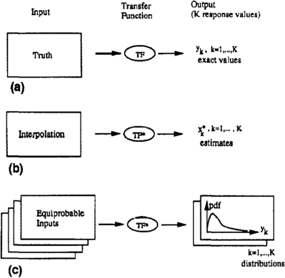
The Monte Carlo technique consists of generating many different joint outcomes of random processes (Figure 1c) and then observing the behavior of response values that are functions of these outcomes. Such behavior can be characterized by probability density functions (pdf) of the response variables, as depicted on the right of Figure 1c).[1]
For example, the input variables might be porosity (φ), oil saturation (S0), and a binary indicator (I) set equal to 1 or 0 depending on whether the sample location belongs to a certain pay formation. The unique response value is the volume of oil in place defined by a particular function of the various input variables, called a transfer function (TF). In this example, the transfer function is a summation representing the total volume V.
In the ideal case of exhaustive sampling, the values used as input are known, so the response value is unique and deterministically known. However, in practice, the previous three input quantities (φ, S0, I) are poorly sampled at best, and the unsampled values must be interpolated, as on the left of Figure 1b. In addition, the transfer function itself, as in the case involving flow simulators, is usually a rough approximation of the actual process taking place in the reservoir. Consequently, the resulting response values (there are usually many) are uncertain estimates of the actual values.
If a critical decision is to be made on these estimated response values, such as pursuing the development of a given project, it is essential to evaluate the uncertainty attached to these estimates or, better still, to evaluate the probability distributions of the response values, as shown on the right of Figure 1c.
A Monte Carlo approach to evaluation of these response distributions consists of the following steps:
- Model any aspect of uncertainty about either the input variables or the parameters of the transfer function by use of the concept of random variables. For example, the joint spatial distribution of the three variables porosity, oil saturation, and indicator of formation presence can be modeled by three, usually interdependent, random functions.
- Draw joint realizations (outcomes) of these random variables or functions. Each realization represents an alternative equiprobable input set to the transfer function. Many such realizations could be retained, as on the left of Figure 1c.
- Transfer the input uncertainty through the transfer function into sets of response values. The histogram of the response values provides a probabilistic assessment of the impact of input uncertainty on that response, as shown on the right of Figure 1c.
Step 1 consists of the determination and probabilistic modeling of the most consequential aspects (for the transfer function being considered) of the input uncertainty. Returning to the example of evaluation of oil volume in place, important elements of input uncertainty include the respective spatial continuity in space of the variables porosity, oil saturation, and formation boundaries; the spatial correlation of porosity and saturation; and whether these two variables depend on the proximity of the formation boundaries. Indeed, the greater the spatial continuity of any variable, the smaller (on average) the estimation error when interpolating an unsampled value from neighboring data.
Step 2 consists of drawing realizations (outcomes) from a multivariate set of random functions. These realizations reflect the statistical properties of the random function models (such as histograms and correlograms) in addition to honoring the actual data values at their locations.
Step 3 involves the repetitive application of the transfer function on each of the realizations of the input variables. If that transfer function is a simple, well-defined mathematical function (such as the equation defining the oil volume in place), step 3 poses no particular problem. However, if the transfer function involves a complex flow simulator, repetitive runs of such a transfer function can be tedious if not prohibitive in computer time. Various approximations are then possible, such as streamlining the transfer function, modeling the response distribution(s) from only a limited number of response values, or bounding type approaches in which only some quantiles of the probability distribution of the response values are determined.
The concept of Monte Carlo analysis is generally straightforward and this approach is often used. However, depending on the complexity of the problem, particularly the transfer function being considered, this approach can be quite difficult and time consuming.[2] The small book by Hammersley and Handscomb[3] provides a general discussion of Monte Carlo analysis.
Stochastic simulation

Stochastic simulation is a tool that allows Monte Carlo analysis of spatially distributed input variables. It aims at providing joint outcomes of any set of dependent random variables. These random variables can be
- Discrete (indicating the presence or absence of a character), such as facies type
- Continuous, such as porosity or permeability values
- Random sets, such as ellipses with a given distribution of size and aspect ratio, or shapes drawn at random from a frequency table of recorded shapes
The set of random variables can be any combination of these types. Some random variables can be functions of the geographic coordinates, in which case they are called random functions.
The dependence characteristics of these random variables are usually limited to 2-by-2, or bivariate, dependence, as opposed to k-by-k dependence involving k variables at a time, with k > 2. Bivariate dependence characteristics can be of the simpler linear correlation type, as defined by the correlation coefficient between any two variables. They can also be of the more complete type involving the bivariate probability distribution function.
The joint outcomes must verify any number of, or all of, the following typical conditions:
- All outcomes are equally probable, which does not imply that they are all similar. In particular, one realization can be quite similar to some and still different from others.
- The histogram of the simulated values of any one attribute reasonably reproduces the probability density function of the corresponding random variable model.
- The dependence characteristics between any two random variables are reproduced by the corresponding realizations. These two random variables can relate to the same attribute at two different locations in space or to two different attributes at either the same location or at two different locations.
- All outcomes honor the sample data values.
In a spatial context where all the random variables relate to the same attribute at different locations, condition 4 amounts to honoring the sample values at their locations. This condition is also known as the exactitude condition, and the corresponding realizations are referred as being conditional to the data values.
There are as many algorithms for generating joint realizations of a large number of dependent random variables as there are different models for the joint distribution of these random variables, with an equally large number of implementation variants. With the advent of extremely fast computers with vast memory, the field is exploding with new algorithms being proposed regularly. The book by Ripley[4] gives an excellent summary and an attempt at classification of the algorithms, yet as of 1990, it can no longer be considered complete. A good generic discussion of simulation topics is given in Hohn.[5]
Particular mention should be given to stochastic simulations based on self repetitive fractal models.[6] Such models correspond to patterns of spatial variability that repeat themselves whatever the distance scale used.
The present ability to generate a large number of very large stochastic simulations very quickly far outstrips the capability to look at the corresponding (stochastic) images and the capability to process them with realistic flow simulators. The bottleneck for systematic utilization of the Monte Carlo approach is no longer stochastic simulation but rather computer graphics and flow simulators that are presently much too slow.
See also
References
- ↑ Journel, A. G., 1989, Fundamentals of geostatistics in five lessons: Washington D.C., American Geophysical Union, Short Course in Geology, v. 8, 40 p.
- ↑ Box, G. E. P., and N. R. Draper, 1987, Empirical model building and response surfaces: New York, John Wiley, 669 p.
- ↑ Hammersley, J. M., and D. C. Handscomb, 1964, Monte Carlo methods: Chapman and Hall (reprint 1983), 178 p.
- ↑ Ripley, B. D., 1987, Stochastic Simulation: New York, John Wiley, 237 p.
- ↑ Hohn, M. E., 1988, Geostatistics and petroleum geology: New York, Van Nostrand Reinhold, 264 p.
- ↑ Hewett, T. A., 1986, Fractal distribution of reservoir heterogeneity and their influence on fluid transport: Society of Petroleum Engineers, SPE Paper 15386.