Seismic data preparation for mapping
| Exploring for Oil and Gas Traps | |

| |
| Series | Treatise in Petroleum Geology |
|---|---|
| Part | Predicting the occurrence of oil and gas traps |
| Chapter | Interpreting seismic data |
| Author | Christopher L. Liner |
| Link | Web page |
| Store | AAPG Store |
Before seismic data can be used in maps, they must be checked for quality; they must have reflectors identified for key geologic horizons, which should be tracked throughout the data grid; and key sections must be interpreted structurally.
Example data set
The example given in this section is a small 3-D data set from the Glenn Pool field in northeastern Oklahoma. The target is the Ordovician Wilcox Formation. The interpretation was done using a system called Cubic.
Procedure
Follow the steps listed below to make a classic structural seismic interpretation.
- Preview data for quality and consistency with acquisition and processing reports.
- Make structure contour maps for key horizons using well control only.
- Identify online wells with velocity control.
- Compute a synthetic seismogram for each online well with a sonic or density log.
- Associate reflectors at each online well with stratigraphic horizons using vertical seismic profile (VSP), synthetic seismogram, or time-stretched logs.
- Interpret seismic data using color identifiers (tracking) by extending reflection events across the entire survey area.
- Mark faults and key structural details.
Step 1: Preview data

Preview seismic data for quality and consistency using acquisition and processing reports that come with the data. Note any geological conditions that might cause the interpretation method listed in the procedure to fail. As shown in Figure 1A, each 3-D seismic survey has a unique outline of live traces or image area. Use the outline of the image area with the processing report and well spots (Figure 1B) to confirm correct orientation of the survey. This might sound silly but it is very easy to get the orientation wrong since there are many ways to orient a cube.
Step 2: Create well control maps
A depth structure map should be constructed using all available well control to the horizon of interest. There are many ways of gridding or contouring depth points. Whatever the method, it should also be used in the depth conversion velocity map (next section). The wells-only depth structure map is a useful baseline.
Step 3: Identify wells with velocity control
Identifying online wells with velocity control is a vital point in the seismic mapping process. For a 2-D survey, online wells are located on a seismic line. For a 3-D survey every well in the image area is online. The velocity control can be (in order of preference)
- Vertical seismic profile (VSP)
- Sonic log
- Checkshot survey
Step 4: Compute simulated seismic traces
For each online well with a sonic or density log, we can compute a simulated seismic trace (synthetic seismogram). Another option is to convert sonic log (or velocity, density, velocity * density) to time and directly overlay onto the seismic section being interpreted. Figure 12-8 (from the Glenn Pool survey) shows this approach. For wells with a VSP, a trace is available directly and need not be simulated.
Step 5: Identify stratigraphy of reflectors
Correlate seismic reflectors at each online well with key geological horizons using a VSP or a synthetic seismogram. A checkshot survey can be used as a last resort. Ideally, events should be correlated for every online well.
Step 6: Track events
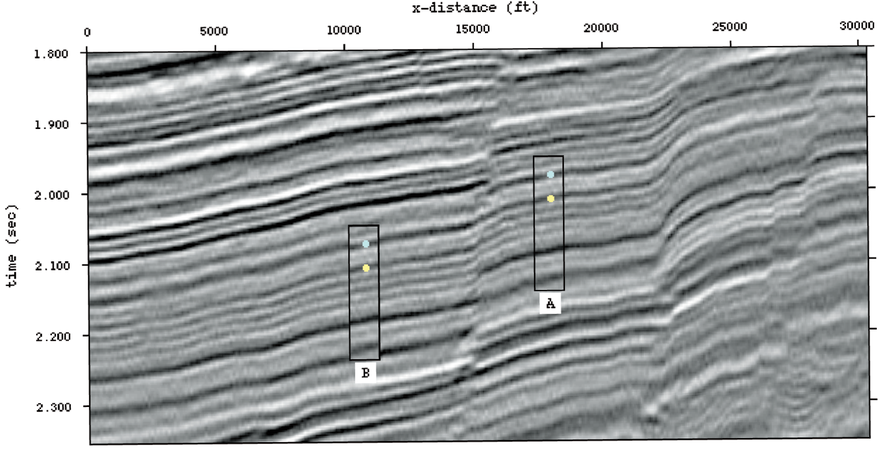
Figure 2 Jump correlation. Copyright: Liner;[1] courtesy PennWell.
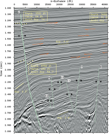
Figure 3 Marked up section. Copyright: Liner;[1] courtesy PennWell.


Interpret seismic data using color identifiers by extending reflection events across the entire survey area. This process is called tracking—following an event throughout the data volume.
Step 7: Mark faults
Mark faults and other structural details on the seismic sections. If necessary, jump-correlate picked events across faults. When a conflict exists, a well-tie correlation is preferred to seismic jump correlation across faults. The seismic section in Figure 2 shows a jump correlation. A small panel of data, labeled A, is outlined on the right side of the fault. Two key horizons are marked. The data panel was copied, then moved across the fault and adjusted until a satisfactory fit was made at B. Note the apparently continuous event connecting the yellow dot at A with the blue dot at B. This is a false correlation.
Marking up key sections
Beyond jump correlation, an important part of structural interpretation is to mark up a few key lines in detail. Figure 3 shows part of such a marked-up section. Faults are marked in green, with line width denoting relative importance. Sense of throw is indicated as up (U) or down (D). Yellow dots indicate events used to calculate depth and fault throw, while yellow lines are events used for dip calculations. Fault numbers indicate relative age (1 = most recently active, etc.). Red arrows show stratigraphic bed terminations. The arrowhead indicates whether termination is from above or below. For depth, throw, and dip estimates, a simple linear velocity model was used: υ(z) = 5,000 + 0.4*z, where υ is in ft/sec and z is depth in feet. This velocity model is often useful in basins that contain unconsolidated sediments, such as the Gulf of Mexico. The data for Figures 2 and 3 come from Southeast Asia.
See also
References
External links
| find literature about Seismic data preparation for mapping |