Difference between revisions of "Synthetic seismogram"
(→See also: reduced list) |
Cwhitehurst (talk | contribs) m (added Category:Methods in Exploration 10 using HotCat) |
||
| (19 intermediate revisions by 3 users not shown) | |||
| Line 13: | Line 13: | ||
| isbn = 0891816607 | | isbn = 0891816607 | ||
}} | }} | ||
| − | The more control the geoscientist has in mapping the subsurface, the greater the accuracy of the maps. Control can be increased by the correlation of seismic data with borehole data. The synthetic seismogram (often called simply the “synthetic”) is the primary means of obtaining this correlation. | + | The more control the geoscientist has in mapping the subsurface, the greater the accuracy of the maps. Control can be increased by the correlation of [[seismic data]] with borehole data. The synthetic seismogram (often called simply the “synthetic”) is the primary means of obtaining this correlation. |
| − | Velocity data from the sonic log (and the density log, if available) are used to create a synthetic seismic trace. This trace closely approximates a trace from a seismic line that passes close to the well in which the logs were acquired. The synthetic then correlates with both the seismic data and the well log from which it was generated. | + | Velocity data from the sonic log (and the [[density log]], if available) are used to create a synthetic seismic trace. This trace closely approximates a trace from a seismic line that passes close to the well in which the logs were acquired. The synthetic then correlates with both the seismic data and the well log from which it was generated. |
| − | ==Calculating | + | ==Calculating a synthetic seismogram== |
| + | |||
| + | [[file:synthetic-seismograms_fig1.png|400px|thumb|{{figure number|1}}Synthetic seismogram and associated well log data.]] | ||
The calculation of a synthetic seismogram generally follows these steps: | The calculation of a synthetic seismogram generally follows these steps: | ||
| Line 26: | Line 28: | ||
* A wavelet is chosen that has a frequency response and band width similar to that of the nearby seismic data. The synthetic wavelet is convolved with the reflection series for the entire well survey and generates a synthetic seismic trace. A potential pitfall in synthetic generation is using a wavelet of fixed frequency over the entire survey. Care should be taken to choose a wavelet whose frequency is similar to a key interval of the seismic data to which it will be compared. | * A wavelet is chosen that has a frequency response and band width similar to that of the nearby seismic data. The synthetic wavelet is convolved with the reflection series for the entire well survey and generates a synthetic seismic trace. A potential pitfall in synthetic generation is using a wavelet of fixed frequency over the entire survey. Care should be taken to choose a wavelet whose frequency is similar to a key interval of the seismic data to which it will be compared. | ||
| − | The resulting trace is displayed at the same vertical scale as the seismic section for direct comparison. To improve the match with the seismic data, the synthetic seismic trace can be recomputed using different wavelets and filters. Figure 1 shows an example of a synthetic seismogram and associated well log data used in its generation. Different wavelets have been convolved to produce two additional synthetic seismogram displays. | + | The resulting trace is displayed at the same vertical scale as the seismic section for direct comparison. To improve the match with the seismic data, the synthetic seismic trace can be recomputed using different wavelets and filters. [[:file:synthetic-seismograms_fig1.png|Figure 1]] shows an example of a synthetic seismogram and associated well log data used in its generation. Different wavelets have been convolved to produce two additional synthetic seismogram displays. |
| + | |||
| + | The synthetic trace can now be compared to a trace from the seismic line. This is commonly done by laying the synthetic directly on top of the appropriate seismic trace and adjusting the synthetic vertically until the two coincide. Through a trial-and-error process, the interpreter determines at what point the synthetic trace “best fits” the seismic data. | ||
| + | |||
| + | In an ideal world, there is an obvious agreement between the seismic line trace and the synthetic seismogram. A formation top or other correlation marker on the well log can then be tied to the corresponding seismic horizon with relative ease. In the real world, however, the interpreter may be, and often is, confronted with a synthetic trace and seismic data trace that bear little resemblance to each other. Variations in the quality of the well log data can have a major impact on the final synthetic display. A sonic log that was generated from a borehole containing numerous washed out zones will contain areas of unrealistic velocities. Careful editing of the well log data can help to smooth spurious data readings and generate a more realistic synthetic. Care should be taken, however, whenever well log data are edited. For more details about synthetic seismograms, the interested reader can refer to ''Seismic Exploration Fundamentals'' ([[Coffen, 1978]]).{{Citation needed}} | ||
| + | |||
| + | ==Creating a synthetic seismogram== | ||
| + | {{publication | ||
| + | | image = exploring-for-oil-and-gas-traps.png | ||
| + | | width = 120px | ||
| + | | series = Treatise in Petroleum Geology | ||
| + | | title = Exploring for Oil and Gas Traps | ||
| + | | part = Predicting the occurrence of oil and gas traps | ||
| + | | chapter = Interpreting seismic data | ||
| + | | frompg = 12-1 | ||
| + | | topg = 12-29 | ||
| + | | author = Christopher L. Liner | ||
| + | | link = http://archives.datapages.com/data/specpubs/beaumont/ch12/ch12.htm | ||
| + | | pdf = | ||
| + | | store = http://store.aapg.org/detail.aspx?id=545 | ||
| + | | isbn = 0-89181-602-X | ||
| + | }} | ||
| + | Once a stratigraphic model has been built using velocities and densities, a synthetic seismogram (or synthetic) can be constructed to identify seismic reflections. A synthetic seismogram is the fundamental link between well data and [[seismic data]], and it is the main tool (along with a [[Checkshots_and_vertical_seismic_profiles#Vertical_seismic_profiles|vertical seismic profile [VSP]]], if available) that allows geological picks to be associated with reflections in the seismic data. As discussed, if a VSP is available for a particular well, a synthetic is not needed. The VSP directly measures both time and depth to a formation of interest. Usually synthetic seismograms are created using specialized software. The user may be unaware of the process that creates them. The steps necessary to create a synthetic seismogram manually are described below: | ||
| + | |||
| + | # Edit the sonic and density logs for bad intervals. | ||
| + | # Calculate vertical reflection times. | ||
| + | # Calculate reflection coefficients, R<sub>o</sub> . | ||
| + | # Combine the last two items to create a reflection coefficient time series. | ||
| + | # Convolve the reflection coefficient series with the wavelet. | ||
| + | |||
| + | ==Reflection coefficient== | ||
| + | The normal-incidence reflection coefficient for a rock contact is an important quantity. Sheriff (1984) defines it as “the ratio of the amplitude of the displacement of a reflected wave to that of the incident wave.” Mathematically, reflection coefficient can be expressed as | ||
| − | + | :<math>R_{0} = \frac{(\rho_{2} \upsilon_{2} - \rho_{1} \upsilon_{1})}{(\rho_{2} \upsilon_{2} + \rho_{1} \upsilon_{1})}</math> | |
| − | The | + | where: |
| + | |||
| + | * ρ = rock density | ||
| + | * ''υ'' = rock velocity | ||
| + | * 1 = parameters above the interface | ||
| + | * 2 = parameters below the interface | ||
| + | |||
| + | ==Convolutional model== | ||
| + | The final simulated seismic trace can be summarized by the convolutional model: | ||
| + | |||
| + | :<math>T(t) = R_{0}(t) \times w(t) + n(t)</math> | ||
| + | |||
| + | where: | ||
| + | |||
| + | * ''T''(''t'') = seismic trace | ||
| + | * ''R''<sub>0</sub>(''t'') = reflection coefficient series (spikes) | ||
| + | * * = convolution | ||
| + | * ''w''(''t'') = wavelet | ||
| + | * ''n''(''t'') = noise | ||
| + | |||
| + | This model of the seismic trace assumes many things, including removal of all amplitude effects except R<sub>0</sub>. The job of seismic data processors is to deliver data to the interpreter in a form consistent with the convolutional model, but it is hard to get it right. | ||
| + | |||
| + | ==Example synthetic seismogram== | ||
| + | [[file:interpreting-seismic-data_fig12-7.png|300px|thumb|{{figure number|2}}Simple synthetic seismogram. From software by S. Hill, Conoco.]] | ||
| − | + | [[:file:interpreting-seismic-data_fig12-7.png|Figure 2]] shows a simple synthetic seismogram. We can see most of the components that go into the creation of a synthetic seismogram—the velocity model, reflection coefficient series, individual wavelets, synthetic trace, and simulated stack section (lower plot). The velocity model is from north-central Oklahoma. The density model is not shown. | |
==See also== | ==See also== | ||
| + | * [[Seismic data: building a stratigraphic model]] | ||
| + | * [[Synthetic seismograms: correlation to other data]] | ||
| + | * [[Seismic data: identifying reflectors]] | ||
* [[Seismic interpretation]] | * [[Seismic interpretation]] | ||
* [[Vertical and lateral seismic resolution and attenuation]] | * [[Vertical and lateral seismic resolution and attenuation]] | ||
| Line 46: | Line 105: | ||
* [http://store.aapg.org/detail.aspx?id=612 Find the book in the AAPG Store] | * [http://store.aapg.org/detail.aspx?id=612 Find the book in the AAPG Store] | ||
| − | [[Category:Geophysical methods]] | + | [[Category:Geophysical methods]][[Category:Interpreting seismic data]] |
| + | [[Category:Methods in Exploration 10]] | ||
Latest revision as of 13:57, 24 January 2022
| Development Geology Reference Manual | |

| |
| Series | Methods in Exploration |
|---|---|
| Part | Geophysical methods |
| Chapter | Synthetic seismograms |
| Author | Kari Rekoske, David Hicks |
| Link | Web page |
| Store | AAPG Store |
The more control the geoscientist has in mapping the subsurface, the greater the accuracy of the maps. Control can be increased by the correlation of seismic data with borehole data. The synthetic seismogram (often called simply the “synthetic”) is the primary means of obtaining this correlation.
Velocity data from the sonic log (and the density log, if available) are used to create a synthetic seismic trace. This trace closely approximates a trace from a seismic line that passes close to the well in which the logs were acquired. The synthetic then correlates with both the seismic data and the well log from which it was generated.
Calculating a synthetic seismogram
The calculation of a synthetic seismogram generally follows these steps:
- The sonic and density curves are digitized at a sample interval of 0.5 to length::1 ft. (If the density curve is not available, the sonic alone may be used.)
- A computer program computes the acoustic impedance log from the sonic velocities and the density data. The data are often averaged or “blocked” to larger sample intervals to reduce computation time and to smooth them without aliasing the log values.
- The resulting acoustic impedance curve is then used by the program to compute reflection coefficients at each interface between contrasting velocities.
- A wavelet is chosen that has a frequency response and band width similar to that of the nearby seismic data. The synthetic wavelet is convolved with the reflection series for the entire well survey and generates a synthetic seismic trace. A potential pitfall in synthetic generation is using a wavelet of fixed frequency over the entire survey. Care should be taken to choose a wavelet whose frequency is similar to a key interval of the seismic data to which it will be compared.
The resulting trace is displayed at the same vertical scale as the seismic section for direct comparison. To improve the match with the seismic data, the synthetic seismic trace can be recomputed using different wavelets and filters. Figure 1 shows an example of a synthetic seismogram and associated well log data used in its generation. Different wavelets have been convolved to produce two additional synthetic seismogram displays.
The synthetic trace can now be compared to a trace from the seismic line. This is commonly done by laying the synthetic directly on top of the appropriate seismic trace and adjusting the synthetic vertically until the two coincide. Through a trial-and-error process, the interpreter determines at what point the synthetic trace “best fits” the seismic data.
In an ideal world, there is an obvious agreement between the seismic line trace and the synthetic seismogram. A formation top or other correlation marker on the well log can then be tied to the corresponding seismic horizon with relative ease. In the real world, however, the interpreter may be, and often is, confronted with a synthetic trace and seismic data trace that bear little resemblance to each other. Variations in the quality of the well log data can have a major impact on the final synthetic display. A sonic log that was generated from a borehole containing numerous washed out zones will contain areas of unrealistic velocities. Careful editing of the well log data can help to smooth spurious data readings and generate a more realistic synthetic. Care should be taken, however, whenever well log data are edited. For more details about synthetic seismograms, the interested reader can refer to Seismic Exploration Fundamentals (Coffen, 1978).[citation needed]
Creating a synthetic seismogram
| Exploring for Oil and Gas Traps | |

| |
| Series | Treatise in Petroleum Geology |
|---|---|
| Part | Predicting the occurrence of oil and gas traps |
| Chapter | Interpreting seismic data |
| Author | Christopher L. Liner |
| Link | Web page |
| Store | AAPG Store |
Once a stratigraphic model has been built using velocities and densities, a synthetic seismogram (or synthetic) can be constructed to identify seismic reflections. A synthetic seismogram is the fundamental link between well data and seismic data, and it is the main tool (along with a vertical seismic profile [VSP], if available) that allows geological picks to be associated with reflections in the seismic data. As discussed, if a VSP is available for a particular well, a synthetic is not needed. The VSP directly measures both time and depth to a formation of interest. Usually synthetic seismograms are created using specialized software. The user may be unaware of the process that creates them. The steps necessary to create a synthetic seismogram manually are described below:
- Edit the sonic and density logs for bad intervals.
- Calculate vertical reflection times.
- Calculate reflection coefficients, Ro .
- Combine the last two items to create a reflection coefficient time series.
- Convolve the reflection coefficient series with the wavelet.
Reflection coefficient
The normal-incidence reflection coefficient for a rock contact is an important quantity. Sheriff (1984) defines it as “the ratio of the amplitude of the displacement of a reflected wave to that of the incident wave.” Mathematically, reflection coefficient can be expressed as
where:
- ρ = rock density
- υ = rock velocity
- 1 = parameters above the interface
- 2 = parameters below the interface
Convolutional model
The final simulated seismic trace can be summarized by the convolutional model:
where:
- T(t) = seismic trace
- R0(t) = reflection coefficient series (spikes)
- * = convolution
- w(t) = wavelet
- n(t) = noise
This model of the seismic trace assumes many things, including removal of all amplitude effects except R0. The job of seismic data processors is to deliver data to the interpreter in a form consistent with the convolutional model, but it is hard to get it right.
Example synthetic seismogram
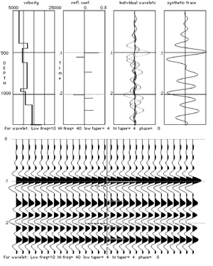
Figure 2 shows a simple synthetic seismogram. We can see most of the components that go into the creation of a synthetic seismogram—the velocity model, reflection coefficient series, individual wavelets, synthetic trace, and simulated stack section (lower plot). The velocity model is from north-central Oklahoma. The density model is not shown.
See also
- Seismic data: building a stratigraphic model
- Synthetic seismograms: correlation to other data
- Seismic data: identifying reflectors
- Seismic interpretation
- Vertical and lateral seismic resolution and attenuation
- Forward modeling of seismic data
- Introduction to geophysical methods
- Checkshots and vertical seismic profiles


