Difference between revisions of "Pickett plot construction"
(Initial import) |
Cwhitehurst (talk | contribs) m (added Category:Treatise Handbook 3 using HotCat) |
||
| (14 intermediate revisions by 3 users not shown) | |||
| Line 6: | Line 6: | ||
| part = Predicting the occurrence of oil and gas traps | | part = Predicting the occurrence of oil and gas traps | ||
| chapter = Predicting reservoir system quality and performance | | chapter = Predicting reservoir system quality and performance | ||
| − | | frompg = 9- | + | | frompg = 9-60 |
| − | | topg = 9- | + | | topg = 9-63 |
| author = Dan J. Hartmann, Edward A. Beaumont | | author = Dan J. Hartmann, Edward A. Beaumont | ||
| link = http://archives.datapages.com/data/specpubs/beaumont/ch09/ch09.htm | | link = http://archives.datapages.com/data/specpubs/beaumont/ch09/ch09.htm | ||
| Line 14: | Line 14: | ||
| isbn = 0-89181-602-X | | isbn = 0-89181-602-X | ||
}} | }} | ||
| − | A Pickett plot lets us compare water saturations of different parts of a reservoir in one or many wells. The Pickett plot<ref name=ch09r45>Pickett, G., R., 1973, Pattern recognition as a means of formation evaluation: The Log Analyst, vol. 14, no. 4, p. 3–11.</ref> is a visual representation of the Archie equation and therefore is a powerful graphic technique for estimating S<sub>w</sub> ranges within a reservoir. All that is needed to make a Pickett plot is a set of porosities and corresponding resistivities taken from well logs and 2×4 cycle log-log paper. The procedure for making a Pickett plot consists of five steps, detailed below. | + | A Pickett plot lets us compare water saturations of different parts of a reservoir in one or many wells. The Pickett plot<ref name=ch09r45>Pickett, G., R., 1973, Pattern recognition as a means of formation evaluation: The Log Analyst, vol. 14, no. 4, p. 3–11.</ref> is a visual representation of the [[Archie equation]]<ref name=Archie_1942>Archie, G. E., 1942, The electrical resistivity log as an aid in determining some reservoir characteristics: Petroleum Transactions of AIME 146: 54–62.</ref> and therefore is a powerful graphic technique for estimating S<sub>w</sub> ranges within a reservoir. All that is needed to make a Pickett plot is a set of porosities and corresponding resistivities taken from well logs and 2×4 cycle log-log paper. The procedure for making a Pickett plot consists of five steps, detailed below. |
| − | + | # Plot points of matching [[porosity]] and true resistivity (R<sub>t</sub> ) on log-log paper. | |
| − | + | # Plot R<sub>w</sub> point on the R<sub>t</sub> scale. | |
| − | + | # Determine ''m'' using the table of values. | |
| − | + | # Plot the 100% S<sub>w</sub> line. | |
| − | + | # Plot the lines representing lower values of S<sub>w</sub> . | |
| − | |||
| − | |||
| − | |||
| − | |||
| − | |||
| − | |||
| − | |||
| − | |||
| − | |||
| − | |||
| − | |||
| − | |||
| − | |||
| − | |||
| − | |||
==Step 1: Plot points== | ==Step 1: Plot points== | ||
| − | |||
| − | [[file:predicting-reservoir-system-quality-and-performance_fig9-36.png|thumb|{{figure number| | + | [[file:predicting-reservoir-system-quality-and-performance_fig9-36.png|thumb|300px|{{figure number|1}}Plot points of matching porosity and true resistivity (R<sub>t</sub>) values obtained from well logs on 2×4 cycle log-log paper.]] |
| + | |||
| + | Plot points of matching porosity and true resistivity (R<sub>t</sub>) values obtained from well logs on 2×4 cycle log-log paper, as shown in [[:file:predicting-reservoir-system-quality-and-performance_fig9-36.png|Figure 1]]. Use the x-axis for the resistivity (R<sub>t</sub>) scale and the y-axis for the porosity (Φ) scale. | ||
==Step 2: plot r<sub>w</sub> point== | ==Step 2: plot r<sub>w</sub> point== | ||
| − | |||
| − | [[file:predicting-reservoir-system-quality-and-performance_fig9-37.png|thumb|{{figure number| | + | [[file:predicting-reservoir-system-quality-and-performance_fig9-37.png|300px|thumb|{{figure number|2}}Plot the R<sub>w</sub> value (resistivity of formation water) by plotting the R<sub>w</sub> point along the R<sub>t</sub> scale on the x-axis at the top of the graph grid where porosity is 100%.]] |
| + | |||
| + | Plot the R<sub>w</sub> value (resistivity of formation water) by plotting the R<sub>w</sub> point along the R<sub>t</sub> scale on the x-axis at the top of the graph grid where porosity is 100%, as shown in [[:file:predicting-reservoir-system-quality-and-performance_fig9-37.png|Figure 2]]. R<sub>w</sub> values are published by logging companies, or we can calculate them from the SP log. | ||
==Step 3: Determine ''m''== | ==Step 3: Determine ''m''== | ||
| Line 52: | Line 39: | ||
{| class = "wikitable" | {| class = "wikitable" | ||
|- | |- | ||
| − | ! | + | ! Porosity type || Value for m |
| − | |||
|- | |- | ||
| − | | Sandstones with diagenetic or detrital clay in pores | + | | Sandstones with diagenetic or detrital clay in pores || 1.7–1.8 |
| − | | 1.7–1.8 | ||
|- | |- | ||
| − | | Formations with clean, macro- to micro-sized pore throats (Archie rocks) | + | | Formations with clean, macro- to micro-sized pore throats (Archie rocks) || 2 |
| − | | 2 | ||
|- | |- | ||
| − | | Formations with vuggy porosity (touching to | + | | Formations with vuggy porosity (touching to non touching) || 2.2–3.0 |
| − | | 2.2–3.0 | ||
|} | |} | ||
==Step 4: Plot the 100% S<sub>w</sub> line== | ==Step 4: Plot the 100% S<sub>w</sub> line== | ||
| + | |||
| + | [[file:predicting-reservoir-system-quality-and-performance_fig9-38.png|300px|thumb|{{figure number|3}}How to plot an ''m'' of 2.]] | ||
| + | |||
On a Pickett plot, the value of ''m'' determines the slope of the S<sub>w</sub> lines. The first S<sub>w</sub> line plotted on a Pickett plot is the 100% S<sub>w</sub> line. To plot this line, draw a line with a negative slope equal to ''m'' that begins at the R<sub>w</sub> point. Use a linear scale to measure the slope; for example, go down [[length::1 in.]] and over 2 in. | On a Pickett plot, the value of ''m'' determines the slope of the S<sub>w</sub> lines. The first S<sub>w</sub> line plotted on a Pickett plot is the 100% S<sub>w</sub> line. To plot this line, draw a line with a negative slope equal to ''m'' that begins at the R<sub>w</sub> point. Use a linear scale to measure the slope; for example, go down [[length::1 in.]] and over 2 in. | ||
| − | [[file:predicting-reservoir-system-quality-and-performance_fig9-38.png| | + | [[:file:predicting-reservoir-system-quality-and-performance_fig9-38.png|Figure 3]] shows how to plot an ''m'' of 2. |
| − | + | ==Step 5: plot s<sub>w</sub> lines== | |
| − | + | [[file:predicting-reservoir-system-quality-and-performance_fig9-39.png|300px|thumb|{{figure number|4}}An example of plotting the lower percentages of S<sub>w</sub>.]] | |
| − | |||
| − | + | After plotting the 100% S<sub>w</sub> line, plot the lines representing lower percentages of S<sub>w</sub> using this procedure: | |
| − | |||
| − | |||
| − | |||
| − | |||
| − | |||
| − | |||
| − | |||
| − | |||
| − | |||
| − | |||
| − | |||
| − | |||
| − | |||
| − | |||
| − | |||
| − | |||
| − | + | # Find the intercept of R<sub>t</sub> = 1 and the 100% S<sub>w</sub> line (made in the last procedure). | |
| + | # From this intercept, draw a line parallel to the x-axis across the plot. Any point on this line has the same porosity. | ||
| + | # Where this line passes through R<sub>t</sub> of 2, 4, 6, 8, 14, and 20, draw a series of lines parallel to the 100% S<sub>w</sub> line. | ||
| + | # Points on these lines correspond to S<sub>w</sub> of 71, 50, 41, 35, 27, and 22%. These percentages are calculated from the Archie equation using ''m'' = 2 and ''n'' = 2 at R<sub>t</sub> of 2, 4, 6, 8, 14, and 20. | ||
| − | [[file:predicting-reservoir-system-quality-and-performance_fig9-39.png| | + | [[:file:predicting-reservoir-system-quality-and-performance_fig9-39.png|Figure 4]] is an example of following this procedure. |
==See also== | ==See also== | ||
* [[Determining water saturation]] | * [[Determining water saturation]] | ||
| − | * [[ | + | * [[Archie equation]] |
* [[Determining Rt]] | * [[Determining Rt]] | ||
* [[Calculating Rw from SP logs]] | * [[Calculating Rw from SP logs]] | ||
| Line 113: | Line 85: | ||
[[Category:Predicting the occurrence of oil and gas traps]] | [[Category:Predicting the occurrence of oil and gas traps]] | ||
[[Category:Predicting reservoir system quality and performance]] | [[Category:Predicting reservoir system quality and performance]] | ||
| + | [[Category:Treatise Handbook 3]] | ||
Latest revision as of 16:16, 5 April 2022
| Exploring for Oil and Gas Traps | |

| |
| Series | Treatise in Petroleum Geology |
|---|---|
| Part | Predicting the occurrence of oil and gas traps |
| Chapter | Predicting reservoir system quality and performance |
| Author | Dan J. Hartmann, Edward A. Beaumont |
| Link | Web page |
| Store | AAPG Store |
A Pickett plot lets us compare water saturations of different parts of a reservoir in one or many wells. The Pickett plot[1] is a visual representation of the Archie equation[2] and therefore is a powerful graphic technique for estimating Sw ranges within a reservoir. All that is needed to make a Pickett plot is a set of porosities and corresponding resistivities taken from well logs and 2×4 cycle log-log paper. The procedure for making a Pickett plot consists of five steps, detailed below.
- Plot points of matching porosity and true resistivity (Rt ) on log-log paper.
- Plot Rw point on the Rt scale.
- Determine m using the table of values.
- Plot the 100% Sw line.
- Plot the lines representing lower values of Sw .
Step 1: Plot points
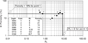
Plot points of matching porosity and true resistivity (Rt) values obtained from well logs on 2×4 cycle log-log paper, as shown in Figure 1. Use the x-axis for the resistivity (Rt) scale and the y-axis for the porosity (Φ) scale.
Step 2: plot rw point
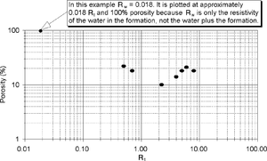
Plot the Rw value (resistivity of formation water) by plotting the Rw point along the Rt scale on the x-axis at the top of the graph grid where porosity is 100%, as shown in Figure 2. Rw values are published by logging companies, or we can calculate them from the SP log.
Step 3: Determine m
Estimate m (cementation factor) using the table below. Laboratory analysis is necessary for a precise determination of m. However, by knowing what the expected porosity type is, we can estimate the value. If you are unsure of the porosity type, use an m of 2.
| Porosity type | Value for m |
|---|---|
| Sandstones with diagenetic or detrital clay in pores | 1.7–1.8 |
| Formations with clean, macro- to micro-sized pore throats (Archie rocks) | 2 |
| Formations with vuggy porosity (touching to non touching) | 2.2–3.0 |
Step 4: Plot the 100% Sw line
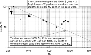
On a Pickett plot, the value of m determines the slope of the Sw lines. The first Sw line plotted on a Pickett plot is the 100% Sw line. To plot this line, draw a line with a negative slope equal to m that begins at the Rw point. Use a linear scale to measure the slope; for example, go down length::1 in. and over 2 in.
Figure 3 shows how to plot an m of 2.
Step 5: plot sw lines
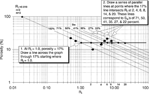
After plotting the 100% Sw line, plot the lines representing lower percentages of Sw using this procedure:
- Find the intercept of Rt = 1 and the 100% Sw line (made in the last procedure).
- From this intercept, draw a line parallel to the x-axis across the plot. Any point on this line has the same porosity.
- Where this line passes through Rt of 2, 4, 6, 8, 14, and 20, draw a series of lines parallel to the 100% Sw line.
- Points on these lines correspond to Sw of 71, 50, 41, 35, 27, and 22%. These percentages are calculated from the Archie equation using m = 2 and n = 2 at Rt of 2, 4, 6, 8, 14, and 20.
Figure 4 is an example of following this procedure.
