Basin modeling: identifying and quantifying significant uncertainties
| Basin Modeling: New Horizons in Research and Applications | |

| |
| Series | Hedberg |
|---|---|
| Chapter | Identifying and Quantifying Significant Uncertainties in Basin Modeling |
| Author | P. J. Hicks Jr., C. M. Fraticelli, J. D. Shosa, M. J. Hardy, and M. B. Townsley |
| Link | Web page |
| Store | AAPG Store |
Introduction
Basin modeling is an increasingly important element of exploration, development, and production workflows. Problems addressed with basin models typically include questions regarding burial history, source maturation, hydrocarbon yields (timing and volume), hydrocarbon migration, hydrocarbon type and quality, reservoir quality, and reservoir pressure and temperature prediction for pre–drill analysis. As computing power and software capabilities increase, the size and complexity of basin models also increase. These larger, more complex models address multiple scales (well to basin) and problems of variable intricacy, making it more important than ever to understand how the uncertainties in input parameters affect model results.
Increasingly complex basin models require an ever-increasing number of input parameters with values that are likely to vary both spatially and temporally. Some of the input parameters that are commonly used in basin models and their potential effect on model results are listed in Table 1. For a basin model to be successful, the modeler must not only determine the most appropriate estimate for the value for each input parameter, but must also understand the range of uncertainty associated with these estimates and the uncertainties related to the assumptions, approximations, and mathematical limitations of the software. This second type of uncertainty may involve fundamental physics that are not adequately modeled by the software and/or the numerical schemes used to solve the underlying partial differential equations. Although these issues are not addressed in this article or by the proposed workflow, basin modelers should be aware of these issues and consider them in any final recommendations or conclusions.
| Property | Effect |
|---|---|
| Depths (or isopachs) | Thickness of each unit controls the relative amount of each rock type (see bulk rock properties) and controls the depth and, therefore, temperature and maturity of each stratigraphic unit. |
| Ages | Ages of each surface and event control timing and thereby control the transient behavior in the model. |
Bulk rock properties
|
The bulk rock properties control the thermal and fluid transport properties (thermal conductivity, density, heat capacity, radiogenic heat, and permeability) that control thermal and pressure evolution in the model. |
| Missing section (erosion) | The amount of missing section controls the burial history of sediments below the associated unconformity. The burial history controls bulk rock properties (primarily thorugh the compaction history) and the temperature and pressure through time. |
| Fluid properties | Fluid properties control bulk rock properties in the porous rocks, migration rates, and affect seal capacity. |
Source properties
|
Source properties control the timing, rate, and fluid type for hydrocarbon generation and expulsion from the source rocks. |
Bottom boundary condition
|
The bottom boundary condition directly affects the temperatures throughout the model. The effects are roughly proportional to depth. |
Top boundary
|
Changes in the top temperature boundary condition affect the steady-state temperature through the model ~1:1. Changes in water depth can affect the top temperature boundary condition and the pressure at the mudline. |
Calibration data
|
The quantity of good calibration data has a direct impact on the quality of the model and the reliability of predictions based on model outputs. |
Considering uncertainty

Uncertainty is present in most, if not all, model inputs and calibration data. These uncertainties generate uncertainties in the model outputs. Sometimes, the resultant uncertainties are not significant enough to impact decisions based on the model results. Other times, these uncertainties can make the model results virtually useless in the decision-making process. Of course, a wide range of cases exist between these extremes, and this is where basin modelers commonly work. In these cases, the model results can be useful, but the uncertainties surrounding the model predictions can be difficult to fully grasp and communicate. Successful decisions based on models in which significant uncertainties exist require that the modeler (1) identify and quantify uncertainties in key input parameters, (2) adequately propagate these uncertainties from input through to output, particularly for three-dimensional models, and (3) clearly communicate this information to decision makers.
Several potential pitfalls can be avoided. Some of the most common are:
- not keeping the goal of the model in mind as it is built to direct and focus the appropriate levels of effort during the model construction
- not clearly identifying which uncertainties in input parameters will have significant impacts on the results and subsequent business decisions
- ignoring the uncertainties because not enough time or a lack of knowledge on how to adequately handle them exists
- working hard on issues that we are comfortable of working on, instead of on those that are truly important
- not recognizing feasible alternative scenarios
Why consider uncertainty? Is not a single deterministic case sufficient for analysis? Consider the simple case of estimating charge volume to a trap. The necessary minimum charge volume required for success (i.e., low charge risk) and a range associated with this minimum charge have been defined and are illustrated by the vertical black solid and dashed lines, respectively, in Figure 1. If a model predicts a charge volume greater than the minimum, then it might be said that little or no charge risk exists. Similarly, if a model predicts a charge volume less than the minimum, then we might say that a significant charge risk exists. These cases are illustrated in Figure 1 and are labeled “low risk” and “high risk,” respectively. However, the perception of what is low risk and what is high risk can change greatly when the probability of an outcome is considered. In this example, the difference between low risk and high risk becomes less definitive, as indicated in Figure 1. Although this is a simplistic illustration, all of the key input parameters in a basin model have the potential to cause this degree of ambiguity in the final results. For that reason, estimates of the range of possible outcomes are as important to the final analysis as estimates of the most likely outcome.
Handling uncertainty
The degree of effort required to adequately handle uncertainty will vary for different parameters and model objectives. In thinking about how to quantify uncertainty, it is commonly useful to divide input parameters into two groups: (1) scalars and (2) maps and volumes. Assigning and propagating uncertainties in scalar values is rather straightforward; assigning and propagating uncertainties in maps and volumes is far less straightforward.
Examples of scalars in a model are the age of a surface or an event or the coefficient in a rock property equation (e.g., compaction, thermal conductivity, or permeability). Probability distribution functions can be used to describe most likely values and the estimated range of scalar values. These distribution functions are used to describe the range and likelihood of values and then to propagate the described uncertainty through a basin model. Simple distributions such as uniform (rectangular), triangular, normal, and log normal are commonly used, but any distribution can be used as long as it honors the observed data while properly accounting for any dependencies.
Examples of maps and volumes include depth surfaces (including paleo–water depths), facies distributions, and basal heat-flow maps. In general, quantifying uncertainties in maps and volumes is much more difficult than quantifying uncertainty in scalars because they consist of multiple values and the spatial dependencies of these values are commonly not easily characterized. Varying each location in a map or volume independently of others is not an ideal solution as this does not consider spatial dependencies. Several approaches have been used in the industry to address the issues associated with maps and volumes. These approaches include simple additive and multiplicative factors, geostatistical approaches, forward modeling, and weighting of multiple scenarios.
Consider two common cases: (1) uncertainty in the depth to a surface generated during a two-dimensional seismic interpretation and (2) uncertainty in the distribution of lithologies within an isopach. Various approaches are available to address each case. In the first case, three primary sources of uncertainty are present: (1) picking the correct surface from the seismic and carrying it throughout the data, (2) interpolation of the surface between the data constraints, and (3) the time-to-depth conversion. In the second case, a different set of uncertainty issues present themselves. Uncertainty in the values of the facies properties and uncertainty in the spatial distribution of those values exist.
Options for handling uncertainty in the depth to a surface might include using a stochastic additive or multiplicative factor to handle uncertainties in interval velocities and interpolation uncertainties using a conditional geostatistical technique (such as Gaussian simulation) to handle estimation away from well control and/or generating multiple scenarios to handle uncertainty in interpretation. Options for handling uncertainty in the distribution of lithologies might include using a conditional geostatistical technique to handle estimation away from data control, forward modeling to handle extrapolation to areas with no data control, and generation of multiple scenarios to handle uncertainty in interpretation and understanding. The best approach in any given situation depends on the type of input parameter under consideration and the available data.
Approach
The workflow presented involves the following steps:
Step 1: Identify the purpose(s) of the model.
Step 2: Develop a base-case scenario.
- The objective of this step is to build a base-case model to be used in subsequent sensitivity analyses.
Step 3: Identify input parameters whose uncertainty might affect the output property of interest and estimate the preliminary ranges of uncertainty for these input parameters.
Step 4: Perform screening simulations to identify key input parameters.
- In the screening step, the parameters whose uncertainty has a significant effect on the output property of interest are identified. The output property of interest should be selected with care and in light of the overall objective of the modeling exercise. For example, given the same model, the key uncertainties are likely to be different depending on whether prediction of overpressure, hydrocarbon charge, or oil quality motivated the construction of the model. The method involves conducting a set of deterministic simulations where each parameter is independently varied from the minimum to the maximum value. The results are plotted using a tornado or similar plot to aid in identification of parameters whose uncertainty has the greatest effect on the desired result. In this evaluation, it is important to consider potential nonlinearities in parameter behavior and to reevaluate the notional base-case model created in step 2.
Step 5: Evaluate the range of uncertainty in key input parameters.
- Once the key parameters have been identified, uncertainties in these parameters are quantified and assigned. The quantification in this step is generally more rigorous than in step 3 (preliminary screening). Quantification typically involves selecting and populating a probability distribution (e.g., uniform, triangular, normal) for each of the key input parameters identified.
Step 6: Propagate the uncertainty in key input parameters through to the output properties of interest via Monte Carlo or similar analysis.
- The final step is a Monte Carlo simulation where values for the input parameters identified in step 4 are randomly selected from the distributions assigned in step 5. The key results from each realization are saved for subsequent evaluation.
Step 7: Iterate as needed to fine tune the input parameters and dependencies between input parameters, to fine tune error bars and weights for calibration data, and to improve the base-case scenario.
- Although several approaches could be used to quantify uncertainty in models, the approach presented uses Monte Carlo simulation. Monte Carlo simulation has the advantage of being (1) able to handle any probability distribution function, (2) able to account for dependencies between variables, and (3) straightforward to implement. It is also typically straightforward to analyze the results of the Monte Carlo simulation. The disadvantages include that it may require a large number of realizations to adequately sample the possible solution space, and it may be difficult to adequately develop probability distribution functions or the required realizations, particularly for maps and volumes.
Hypothetical example
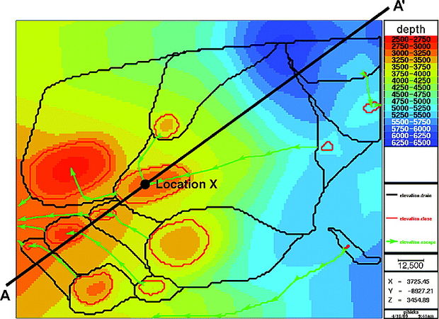
Figure 2 Present-day depth structure map (meters) of the key migration surface. The outlines of the drainage polygons are shown in black, the closures are outlined in red, and the escape paths are shown in green. The scale bar in the legend represents 12,500 m (41,010 ft).
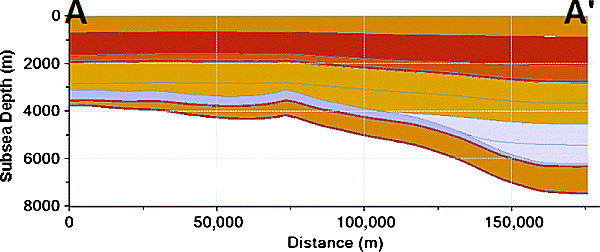
Figure 3 Cross section through the model along the line AA' shown in Figure 2.
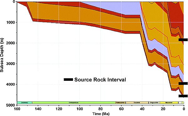
Figure 4 Burial history curve for location X represented by the dot in Figure 2. Source rocks are in the middle of each indicated isopachs.


A hypothetical example is presented to illustrate the approach described. Although the geology is synthetic, it was constructed with realistic basin modeling issues in mind. In this example, the traps of interest formed about 15 Ma. The primary question addressed by the model is, “What is the volume of oil charge to each of the traps during the last 15 m.y.?”
For the purposes of this illustration, the migration analysis has been simplified, and it has been assumed that a present-day map-based drainage analysis is sufficient. A map view of the key surface for the map-based drainage analysis is shown in Figure 2, and a cross section through the model is shown in Figure 3. A burial history curve at location X in Figure 2 is shown in Figure 4. Also shown in Figure 4 are three potential hydrocarbon source rocks, Upper Jurassic, Lower Cretaceous, and lower Miocene. The sources are modeled as uniformly distributed marine source rocks with some terrigenous input.
Step 1: identify the purpose of the model
As previously stated, the purpose of this model is to estimate the volume of oil charge to individual traps during the last 15 m.y.
Step 2: develop a base-case scenario

The next step is to develop and calibrate a base-case scenario. Values for the selected parameters used in this example are listed in the "Most Likely" column of Table 2. In this hypothetical model, only one calibration point is present, so a match to the data is relatively straightforward, but is also nonunique (Figure 5). The uncertainty around the single temperature measurement (±15°C) is indicated by the error bars.
| Property | Minimum | Most Likely | Maximum |
|---|---|---|---|
| Surface temperature (°C) | 10 | 20 | 25 |
| Age of rift (Ma) | 40 | 50 | 60 |
| Duration of rift (m.y.) | 5 | 10 | 20 |
| Background heat flow (mW/m2) | 40 | 50 | 60 |
| Magnitude of extension (γ, 0-1) | 0.1 | 0.64 | 0.9 |
| Shale conductivity (W/m.K) | 1.87 | 2.34 | 2.81 |
| Shale heat generation (mW/m3) | 1.0 | 2.1 | 4.1 |
| Lithology of upper Miocene and Pliocene-Pleistocene isopachs | 10% less shale; 10% more sand | Base | 30% more shale; 30% less sand |
| Depths | 10% shallower | Base | 10% deeper |
| Missing section | - | - | - |
| Upper Miocene (m) | 10 | 100 | 1000 |
| Lower Oligocene (m) | 10 | 100 | 1 |
| Source properties (all 3 sources) | - | - | - |
| Location within isopach | 10% from top | Middle | 90% from top |
| Net thickness (m) | 15 | 30 | 60 |
| oHI (mg-HC/g oTOC)2 | 500 | 600 | 700 |
| oTOC (%)2 | 4 | 4 | 4 |
| OMT lower Miocene source (type II %/type III %)2 | 50/50 | 90/10 | 100/0 |
| OMT other 2 sources (type II %/type III %)2 | 80/20 | 90/10 | 100/0 |
1The base case used the "Most Likely" values. The "Minimum" and "Maximum" values were used in the screening step and as bounds on the Monte Carlo distributions. 2oHI = original hydrogen index of the source rock; oTOC = original total organic carbon content of the source rock; OMT = organic matter type of the source rock.
Step 3: identify and estimate uncertainty in input parameters
In addition to the uncertainties in source type, kinetics, and thickness, it is hypothesized that uncertainties in the depths, amount of missing (eroded) section, lithology (rock properties), shale grain conductivity, radiogenic heat contribution, surface temperature, and basal heat flow (magnitude and timing of extension) could significantly affect the outcome of the model. The estimations of uncertainty in these input parameters are listed in the “Minimum” and “Maximum” columns in Table 2.
Step 4: perform screening simulations to identify key input parameters
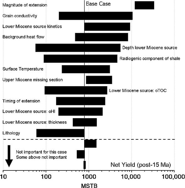
Figure 6 Tornado chart for total net oil yields in million stock tank barrels (MSTB) in a selected drainage polygon during the last 15 m.y. The parameters are sorted by the range of net yields (on a linear scale) for each parameter. Uncertainties in net yields caused by uncertainty in the parameters shown below the horizontal dashed line are too small to be important. Uncertainties in net yields caused by the uncertainty in the parameters for some of the parameters shown above the horizontal line may also be unimportant, particularly for ranges with high low sides. oTOC = original total organic carbon; oHI = original hydrogen index.
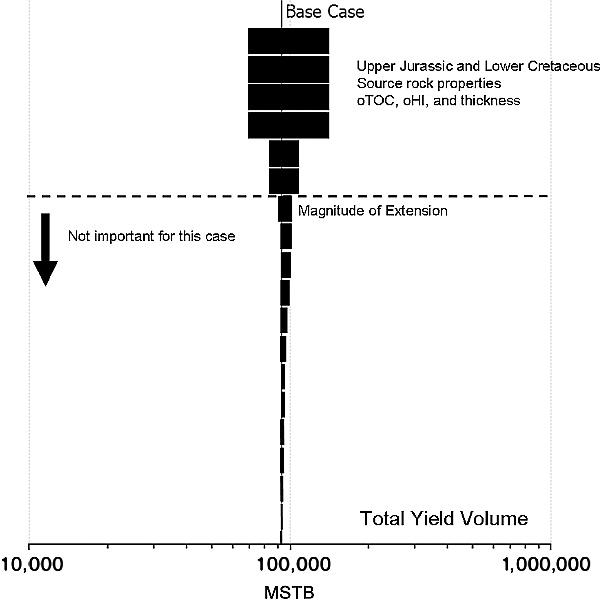
Figure 7 Tornado chart for total yield (million stock tank barrels [MSTB]). In this example, uncertainties in the properties of the Upper Jurassic and Lower Cretaceous source rocks have the most effect on the total oil yield. oTOC and oHI are the original source rock total organic carbon and hydrogen index, respectively. oTOC = original total organic carbon; oHI = original hydrogen index.


Evaluating the sensitivity of results to individual parameters involves exploring the solution space by running a series of basin model simulations in which each parameter is set equal to the maximum value and then to the minimum value while all of the other parameters are held at their base-case value. This process results in 2N + 1 realizations, where N is the number of parameters for which ranges have been defined. In this example, uncertainties were defined for the surface temperature, the magnitude, age, and duration of the rifting event, the background heat flow, the shale conductivity and radiogenic heat generation, the lithology of the upper Miocene and Pliocene isopachs, the depths, the missing section, and the generative characteristics of all three source rocks. These uncertainties are summarized in the "Minimum" and "Maximum" columns of Table 2.
The simulation results are summarized in a tornado chart (Figure 6). The yields are plotted on a log scale to more clearly examine the low-yield (high-risk) cases. Analysis of this plot provides a good opportunity to think about the problem. What properties are important? How important are they? Are there any surprises? The basin modeler should spend some time evaluating the behavior of each parameter to make sure it is understood and makes geologic sense. A limitation of this process is that it does not account for dependencies between input parameters. Thus, the modeler should also give potential dependencies some thought. Examples include a positive correlation between the source rock total organic carbon and hydrogen index, between the mudline temperature and paleo–water depth, between the ages and thickness of isopachs and the timing and magnitude of extension, and between the stratigraphy and paleo–water depths.
Modelers should realize that although it is possible in this sort of analysis for some of these scenarios to be inconsistent with the calibration data, a mismatch on its own is not sufficient reason to narrow the range of values for one of these variables. A particular value of one parameter can cause a mismatch with the data because the value of another parameter is incorrect. If both values were set appropriately, then the model results might be consistent with the calibration data. These interdependency issues will be discussed in more detail later.
The parameters in a tornado plot are sorted by decreasing the range of the net yield resulting from the range given to each input parameter. By constructing the plot in this way, the input parameter uncertainties producing the greatest range in model results are at the top. Twenty-six different parameters were varied in this run; only the 16 parameters with the widest range are shown in Figure 6. The uncertainties associated with the bottom three parameters, and the 10 not shown, are not significant enough to justify the additional effort. Even the uncertainty in some of those “above the line” might not warrant further work. This is because sorting by the widest range does not necessarily equate to sorting by the most important impact on the decisions made based on the results. In this example, the concern is oil yield, so a better sorting might be by the minimum oil yield. In this case, the depth of the Miocene source rock, radiogenic component of the shale, the original total organic carbon in the Miocene source, and the lithology of the Miocene–Pliocene section could be considered the most important, especially if the minimum value of oil yield required for success was on the order of 100 million stock tank barrels (MSTB). The other parameters may not warrant further work or resources.
As mentioned, it is important to remember the question(s) that are being addressed when building a basin model and deciding what input parameters need the most attention. Figure 7 shows the tornado plot for the total expelled hydrocarbon yield as opposed to the net hydrocarbon yield expelled during the last 15 m.y. (Figure 6). Little similarity exists between the parameters that are the most important in these two cases. For the net yields, understanding the timing is critical. For the case in which the total yield is the output property of interest, the generative potential of the Cretaceous and Jurassic sources is more critical than the generative potential of the Miocene source rock.
Although we commonly build our models to address a particular question, in a world of limited time and resources, models can be used for multiple purposes, including purposes that were not originally envisioned at the time the models were constructed. In cases where a model is used for a purpose for which it was not originally built, the modeler should always reexamine the uncertainty in the inputs in light of the new questions being asked.
Nonlinear behavior
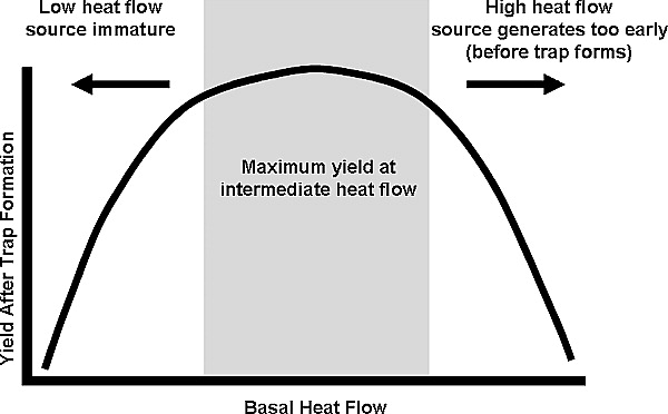
Figure 8 Schematic diagram showing calculated hydrocarbon yields after trap formation as a function of heat flow. At a low heat flow, the source is immature present day and a limited amount of hydrocarbon is generated, and at a high heat flow, the source rock is depleted before the trap forms.
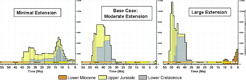
Figure 9 Yield timing for minimum, base, and maximum extension cases for the hypothetical model. In the minimum extension case, the Cretaceous and Jurassic source rocks expel during the last 15 m.y. In the base case, the Cretaceous and Jurassic source rocks are depleted by about 25 Ma, and the Miocene source barely starts generating during the last 2 m.y. In the large extension case, the Cretaceous and Jurassic source rocks are depleted, and the Miocene source rock is generating oil.
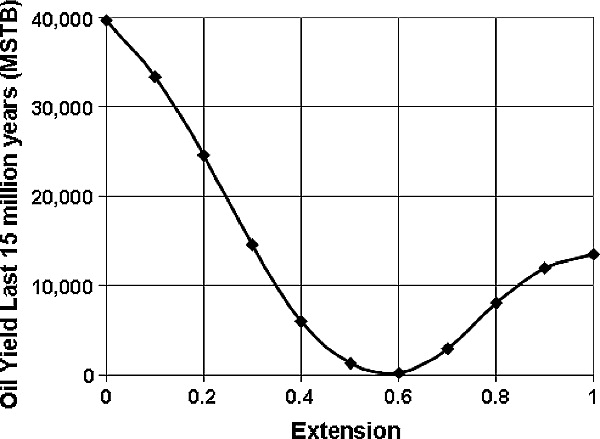
Figure 10 Net yields (last 15 m.y.) as a function of the magnitude of extension.


Commonly, when looking at yields or charge, the behavior is nonlinear and at first glance may not be intuitive. In this example, the magnitude of the extension and the amount of lower Miocene missing section do not, as might be expected, bracket the base case. That is, the post-15 Ma yields are higher than the base case for both the minimum and maximum input values. Consider the straightforward nonlinear relationship between hydrocarbon yield after trap formation and the basal heat flow illustrated in Figure 8. At a low heat flow, the source rock is immature and too little hydrocarbons are generated, and at a high heat flow, the source rock is depleted before the trap forms. This behavior is clearly nonlinear because both high– and low–heat flow scenarios can generate less yield than the base case. However, in the example case presented, the relationship between yield and basal heat flow is the opposite, both high– and low–heat flow cases generate more yield than the base case. This seemingly nonintuitive behavior is a consequence of the inclusion of multiple source rocks in the model and becomes clear when we examine the yield for the three extension cases in detail (Figure 9).
In the base case, the Cretaceous and Jurassic source rocks are depleted by about 25 Ma, and the Miocene source rock barely starts generating during the last 2 m.y. In the minimal extension case, the yield from the Cretaceous and Jurassic source rocks is delayed (relative to the base case) so a significant amount of generation from the Cretaceous and Jurassic sources occurs during the last 15 m.y. In the large extension case, the Cretaceous and Jurassic source rocks are depleted by about 35 Ma, before trap formation, and Miocene source rocks begin generating at 12 Ma instead of at 2 Ma. The net result is that in the base case, little post–trap formation net yield occurs. Volumes of post–trap formation yield are greater than the base case yield in both the minimal and large extension cases. Calculating post–15 Ma hydrocarbon yield as a function of extension allows this effect to be illustrated clearly (Figure 10).
The behavior of all of the key input parameters should be evaluated in a similar manner. After identifying which parameters have uncertainty that significantly affect the output property of interest and the behavior of each parameter as a result of this uncertainty, the ranges and distributions for these parameters should be examined and analyzed. In this example, the magnitude of extension and the depth to the lower Miocene source rock probably warrant further effort, both in narrowing the range of uncertainty and in refining and gaining confidence in the base case.
Step 5: evaluate the range of uncertainty in key input parameters
After the key parameters have been identified, probability distributions need to be developed for each of these input parameters. Thought should be given to what distribution is appropriate for each parameter. If data are available, they should be considered in determining the best distribution. Commonly, distributions are selected based on experience or expert judgment. If any value in the range has about the same chance as another, a uniform distribution is appropriate. If the modeler would like to honor a most likely value, then a triangular or normal distribution or the log version of one of these distributions might be appropriate. In this example, log-triangular distributions were used for the missing section parameters, and triangular distributions were used for the others. The values associated with these distributions are summarized in Table 2.
Step 6: propagate uncertainty to output properties of interest
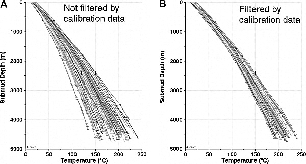
Figure 11 Thermal profiles from 100 Monte Carlo realizations. (A) Results without filtering based on the calibration data. (B) Results with filtering based on the calibration data.
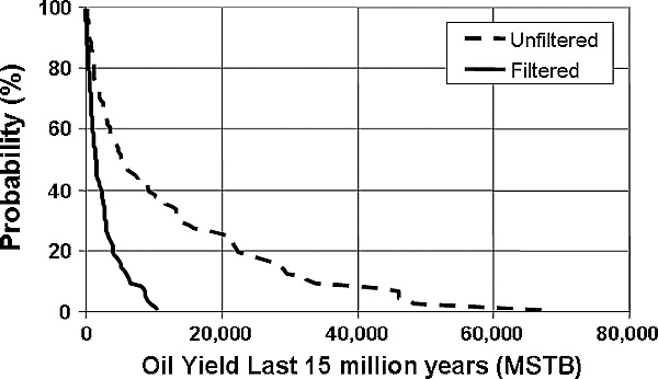
Figure 12 Exceedence probability curves for the oil yield over the last 15 m.y. for a selected drainage polygon for the two cases shown in Figure 11.
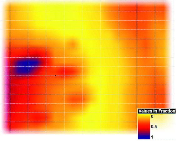
Figure 13 A probability map of net yield greater than 1 million stock tank barrels (MSTB)/km2. Map has the same areal extent as the map in Figure 2.


The goal of this step is to translate the uncertainties in the key input parameters, as described by the probability distribution functions, to uncertainties in the output properties. In the Monte Carlo approach, this translation is accomplished in a brute force manner by calculating a large number of possibilities based on the possible distributions of input parameters. In the absence of calibration data, the results are saved and used to build distributions for the output properties; however, calibration data can be used to show that some realizations are more probable than others.
How should realizations that fall outside the range of the calibration data be handled? One approach would be to reject those realizations as not appropriate. An alternative approach is to accept all realizations, but weight the results based on the fit to the calibration data using a weighting parameter related to the fit to each calibration point. “Fit” in this case is based on a least squares analysis. Both approaches have advantages and drawbacks.
In the example presented, the accept-reject approach is used. The advantages of this approach are (1) it is relatively simple and (2) it forces the modeler to quantitatively think about the quality of specific data points (and possibly adjust the error bars during the calibration or Monte Carlo process). In working the calibration data and associated error bars, the modeler is commonly forced to consider how good (or bad) the data may be. The model may not find acceptable trials if inconsistent data are used. In the example, if another temperature measurement was available (i.e., 150 ± 15°C at 4 km [2.5 mi]), then it would be difficult or even impossible to find realizations that matched both points. This illustrates both the need to calibrate the model before starting the Monte Carlo simulation and the importance of addressing the uncertainty in the calibration data. The error bars on one or both points may need to be changed or the thermal conductivity structure of the model might need to be revised. The primary disadvantages of the accept-reject approach are (1) the artificially sharp line between what is counted and what is rejected and (2) the large number of simulations that may be required to obtain a sufficient number of acceptable realizations. In the above example, a temperature realization that is 14.9°C higher than the calibration point is accepted, but one that is 15.1°C higher is rejected, although they might be considered effectively the same temperature.
The primary advantage of the alternate least squares approach is that it gives more weight to realizations that are better fits to the calibration data. This approach (1) allows explicit weighting of different calibration data, (2) produces no sharp divide between accepted and rejected values, and (3) weights realizations that are better fits to the calibration data more than those that are not. The primary disadvantages of this approach are that (1) it is difficult to build a rigorous objective function (a measure of the fit of the model results to the calibration data) and (2) realizations that are clearly inconsistent with the calibration data will be accepted. The sum of the squares of the residuals (or whatever difference measurement is used) may not be a good measure of the probability that a given model output matches a calibration point because some uncertainty ranges may not be symmetric and, because all realizations are accepted, many unlikely realizations may be accepted. In the additional temperature point example, this alternative approach provides results, but the modeler might not ever recognize that none of the realizations are consistent with both data points. If the same weights were used for each temperature, a most likely result would probably split the difference and not match either point. If the modeler did recognize the issue, it could be addressed by giving the points appropriate weights and/or reevaluating the quality of the calibration data.
The purpose of this article is not to recommend one of these approaches over the other, but to remind the modeler to think about the quality of the calibration data and to understand that multiple approaches are present to incorporate the data. The best option will commonly be problem dependent. For example, a least squares–type approach might be better for weighting a vitrinite reflectance data point from a cuttings sample, where uncertainty exists regarding the measurement, the sample depth, or whether the sample contains reworked material. A reject-accept approach might be better for considering known hydrocarbon accumulations. A spectrum of intermediate cases exists so a hybrid method might prove to be better in some cases than either of the above approaches. For example, there could be some range around each data point that is considered an exact match, a range around that to which some weighting function is applied and then an outer range that is not acceptable.
Figure 11 shows the resulting thermal profiles for 100 realizations of the hypothetical model described. In panel A of Figure 11, the first 100 realizations are accepted. In panel B of Figure 11, the first 100 realizations within the temperature error bars are accepted. In this filtered case example, it is assumed that a reasonable estimate of the accuracy of the single temperature point exists. Given that assumption, realizations outside the error bars are rejected and those inside the error bars are accepted. If the estimate of the accuracy of the temperature data was less precise, the least squares approach might be a good, or even a better, approach. In either case, if the calibration data are to be given any weight, taking all the realizations and weighting them equally would be a poor choice.
The results from a Monte Carlo simulation can be displayed and analyzed in several ways. For example, Figure 12 shows the exceedance probability curves for the yield during the last 15 m.y. for one of the drainage polygons. Curves are shown for both the filtered and unfiltered cases (Figure 11) to illustrate how rejecting realizations that do not honor the observed temperature data affect the exceedance probability. In this example, filtering the simulation results significantly limits the probability of larger oil yields. Figure 13 shows a map of the probability of the oil yield (summed for all three source rocks) during the last 15 m.y. being greater than 1 MSTB/km2. The map shows regions that have a high probability of having generated a specified yield (1 MSTB/km2 in this case), regions that have a low probability, and regions where significant uncertainty exists whether or not a specified yield was generated.
External links
| find literature about Basin modeling: identifying and quantifying significant uncertainties |