Contouring geological data with a computer
| Development Geology Reference Manual | |

| |
| Series | Methods in Exploration |
|---|---|
| Part | Integrated computer methods |
| Chapter | Introduction to contouring geological data with a computer |
| Author | J. L. Gevirtz |
| Link | Web page |
| Store | AAPG Store |
A basic tool for analysis and display of spatial geological data is the contour map. A contour map displays variation of a geological variable, such as thickness, depth, or porosity, over an area of interest with contour lines of equal value. Often, one or more contoured maps form the basis of detailed analysis of potential or actual reservoirs and are used to estimate volumes of fluids contained within pore spaces of the geological feature of interest. These studies require that maps be graphically presentable and that values underlying the graphic representation of the surface be reliable and reproducible. Errors inherent in mathematical estimation procedures must be understood so that reliability of values (volumes, percentages, and so on) obtained from these maps can be estimated.
Shapes of geological surfaces are complex and not readily approximated by simple mathematical functions because they result from a multitude of interacting processes that vary at different spatial scales. Ideally, spatial data should be examined with a spatial sample of regular geometric design. These designs can capture the range of variation exhibited by most spatial phenomena. However, such designs are, for all practical purposes, impossible for most geological work, although in some instances recent developments in satellite imagery allow their economic implementation. In most cases, subsurface geological features are sparsely sampled relative to their complexity and the samples are highly biased to geophysical and/or geological anomalies. Therefore, values of a variable across an area of interest must be estimated by interpolating from a sparse, irregular control point set.
Several control point patterns are commonly encountered in geological practice. These include random patterns or clusters (Figure 1). Geophysical data that contribute to a geological study are gathered in lines. Lines are a special case of clustered points. Each pattern has its own spatial characteristics and must be understood before a meaningful contoured representation can be constructed. Most geological data usually exhibit properties of both end-member patterns. Gridded patterns are rare in geological practice. Most commercial contouring packages compute statistics that when used with visual inspection of the pattern on a base map can greatly aid selection of an appropriate contouring method.
Computer contouring versus hand contouring
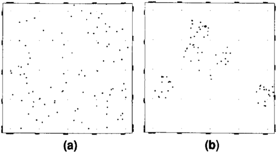
Figure 1 (a) Random points. (b) Clustered points.
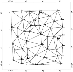
Figure 2 Triangular mesh prepared from Davis'[1] data.
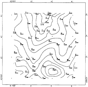
Figure 3 Contoured triangular mesh of Figure 2.
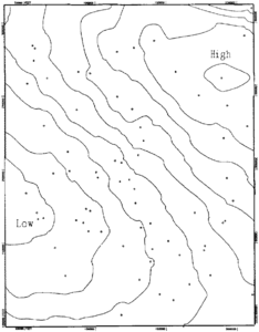
Figure 4 Surface contoured on a triangular mesh. The original surface is a fourth-order polynomial.
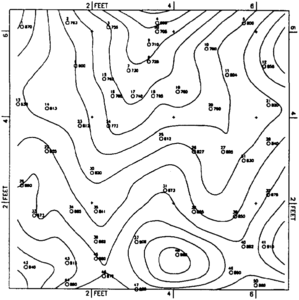
Figure 5 Contours from a 13 × 13 grid using nearest neighbor search. (Data from Davis[1].)
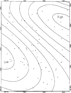
Figure 7 A representation of the fourth-order polynomial of Figure 4 contoured on a grid prepared using a nearest neighbor search criterion.


Contour maps that represent three-dimensional geological surfaces are prepared by time-honored procedures involving estimation methods. Prior to the advent of fast computers and computational algorithms, maps showing geological variation were prepared by hand. Hand-contoured maps represent a geologist's best approximation of the shape of a surface under investigation. Ideas based on the regional geological framework and the geologist's bias arising from prior experience are an inherent part of the hand-contoured map. Hand-contoured maps cannot be reproduced exactly, and values implied by the contours cannot be recovered.
In contrast, high speed computing facilities have engendered methods whereby an “objective” surface can be created by applying mathematical interpolation procedures to a control point set. These methods are free of any geological bias or interpretation introduced during map preparation because they produce a representation of a surface that is constructed by an “unbiased” and decidedly ungeological mathematical formulation from data measured at selected control points. Computer contoured maps can be reproduced easily by presenting the program with the same data and options as those used to create the original map. Values underlying the contoured representation can be obtained by the same interpolation procedure used to generate it.
Procedures usually used in hand contouring require that the geologist choose a contour interval that best displays ideas to be conveyed by the map. Computer-contouring methods, in contrast, require that the geologist select parameters that will ultimately determine the mathematical basis that computes and draws the finished map. Many sets of parameters can be used to produce a contoured representation of a surface sampled by a sparse set of control points. Maps will be similar in overall appearance, but will differ in specific areas because each set of parameters causes different mathematical procedures to be invoked. Each procedure produces a different map. (For example, compare figures 1 and 2 of Phillip and Watson[2] and figure 11.07 of Clarke[3] with Figures 3, 4, 5, and 7 of this article). Suitable parameters for a particular mapping project are selected by carefully inspecting both density and distribution of control points from which the map will be made.
Data values between control points are obtained by some form of interpolation for both manual and computer contouring. For hand-contoured maps, interpolation required to estimate position and shape of individual contours is accomplished by eye or by simple averaging techniques. A triangular mesh or a rectangular grid provide a basis on which to interpolate data from control points. These frameworks rely on a complex mathematical interpolating function (bicubic splines, high order polynomials) to estimate contour positions between data points. This function is a polynomial that is “flexible” and can represent a wide variety of curve shapes. However, these functions have no direct geological significance. They have a continuous derivative everywhere within a triangle or a rectangle and therefore are at least once differentiable. This ensures that slope information implied by the control point set will be more faithfully rendered by the computational procedure.
It is important to recognize that all contouring methods, mathematical or otherwise, are interpolation methods and therefore include error in the resultant surface. This error is related to both the density and location of the measured control points used to construct the surface.
Triangulation
Triangulation connects control points into a mesh of locally equiangular (Delaunay) triangles (Figure 2). Contour positions within the bounds of each triangle are estimated by interpolating from control point values that are triangle vertices. Each member of the triangular mesh is handled separately, and the surface is created by assembling triangles. Interpolation and contouring on a triangulated mesh requires few decisions from the geologist. Control point data are presented to the method along with a contour interval, and a contoured representation of the required surface is produced. Figure 3 is a contour representation of control point data presented by Davis[1] produced by interpolating on a triangular mesh (Figure 2).
Contours prepared on a triangular mesh will always strictly honor all data points used for the interpolation. Triangulated meshes are easily updated, therefore adding new control points and updating maps is simplified. However, contours prepared on this mesh often look “rough” and are less desirable in appearance. Some more sophisticated mapping packages provide smoothing procedures to render maps of more acceptable appearance. Figure 4 is a portion of a surface contoured using a triangulation scheme. Notice the irregular shape of the contours. The original surface that was sampled to produce this map is a fourth order polynomial. The shape of this surface is characterized by smooth contours. Irregularities seen in Figure 4 are artifacts of the interpolation procedure used to estimate the contours within individual triangles. However, the relative positions of the contours are a good approximation to those for the original surface.
Triangulation is not a method of choice when surfaces derived from several horizons for the same area of interest are desired. Operations between surfaces (such as subtraction of the lower from the higher) require that data exist at each control point for both horizons. Often, this is not the case with well data and requires an estimated point to be submitted where data are missing.[4]
Rectangular gridding

Rectangular gridding, in contrast to triangulation, first uses data at measured control points to interpolate values to a set of grid nodes at a predefined spacing. These values are then used to estimate positions of contours crossing each grid rectangle. The complete surface is assembled from contiguous grid rectangles. For most geological applications, grid squares are used rather than the more general rectangle. Interpolation and contouring of an irregularly spaced control point set on a rectangular grid requires many decisions from the geologist.
To obtain a contoured surface representation by a rectangular gridding method, the geologist must decide on a grid spacing, a search criterion, and the method with which to interpolate control point data to grid nodes as well as a suitable contour interval. Most commercial mapping packages include a variety of options for spacing, search criterion, and method. These decisions require an understanding of the relationship between control point density/distribution and the texture of the surface.
Contours resulting from interpolating control point data to equally spaced grid nodes do not strictly honor control points from which they were made because contouring procedures consider estimated values at grid nodes rather than those for the original control points. This can be controlled to some extent by setting a smaller grid spacing. However, smaller grid spacings result in greater interpolation error in sparse data areas so that the map will be aliased by many small features that are artifacts of the gridding procedure itself and have no geological meaning. Setting a suitable grid size requires careful consideration of the distribution and spacing of the control points. Many commercial mapping packages provide average control point distance measures that can be of help when selecting the grid size and search criterion.
Because geological data are rarely presented on a uniform grid and are most often irregularly distributed across the map area, the number of control points used to estimate values at grid nodes is an important consideration. Several search procedures have been devised and are included in most mapping packages. These include nearest neighbor, circular, quadrant, and octant searching.
Nearest neighbor searching uses the nearest neighbors of a grid node to estimate nodal values. The number of neighbors to use can be decided arbitrarily or can be taken as nearest neighbors defined by a Delaunay triangulation of the control point set. The number of nearest neighbors determined from irregularly spaced control points can vary so that each grid node can be estimated from different numbers of control points depending upon their distribution across the map area. Figure 5 is a contour representation of the same data used in Figure 3 using nearest neighbor search and a 13 × 13 grid (Figure 6).
Circular, quadrant, and octant neighborhood searching procedures attempt to balance the number and distribution of control points used to estimate each grid node. Most mapping packages include procedures to estimate density and control point spacing, and these statistics should be examined carefully before deciding on search criteria for a particular project.
Creating a map grid also requires that an interpolation procedure for estimating values at grid nodes be selected. There are numerous methods that have been devised to accomplish this, including weighting methods, trend projection methods, and statistical methods. The more common gridding methods are well summarized by Davis[1] and Clarke.[3]
Weighting methods assign weights to values at control points based on their distance from the grid node being estimated. There are various strategies for devising weighting schemes. The most commonly encountered scheme used for geological data is inverse distance weighting. For this scheme, values at control points are weighted by the inverse of the distance from the node. Variations of this scheme allow the control point values to be weighted by the inverse of distance raised to a selected power. Positive powers cause the influence of more distant points to make a smaller contribution to the value estimated at the grid node. Selection of the power to which the distance is to be raised depends upon the surface “roughness” and a feeling for the relationship between control points and surface shape. Several of these weighting schemes are reviewed by Clarke[3] and Davis.[1]
Trend projection methods are an adaptation of a linear regression technique called trend surface analysis. This method has been devised because geological subsurface sampling rarely provides observations at the highest or lowest points on a surface, and it is sometimes desirable to allow the interpolation procedure to exceed the measured maximum and minimum. Trend projection methods use one of the search criteria previously described to select points that are taken in groups of three and fitted exactly to a plane using a least squares or bicubic spline methods. The grid node estimate is obtained by averaging projections of these planes. This method can be quite effective for smooth surfaces where regional dip orientation remains relatively constant over a large area of the map. This method can produce a surface that is more highly textured than the actual surface in highly deformed areas where the dip direction changes rapidly over small distances. Sampson[5] reviews this method in detail.
Figure 7 is the same portion of the surface shown in Figure 4. The map in Figure 7 was produced by a gridding method with nearest neighbor search. Contours for this map are smooth, and their shape closely approximates those of the original fourth-order polynomial surface from which control points were obtained. However, contours are not in the same geographic positions as in the original surface, and some control points are not strictly honored.
Statistical methods
Several statistical methods can be used to construct a regular grid from control point data. Trend surface analysis is a regression method that fits a power series polynomial to control point data. This method has been used in geological practice to isolate regional trends from sparse control point sets. It is not designed to honor control points, but is used instead to separate regional variation from local variation (for example, separating structural variation from stratigraphic variation). It is often used in exploration, but it has little use in detailed mapping of reservoirs.
Kriging is a statistical method devised by Krige[6] and developed by Matheron,[7] to estimate gold reserves in ore bodies. It has found considerable application as a gridding method in the petroleum industry. The method is based on the theory of the regionalized variable first formulated by Matheron)[7] and popularized by Clark[8] and Journel and Huijbregts.[9] Regionalized variable theory breaks spatial variation into three components. The drift is large-scale variation that can be attributed to regional variation, a smaller scale random but spatially correlated part, and still smaller scale random noise. The method uses knowledge of spatial variance of the drift to derive a set of weights for control points that are unbiased statistical estimates. If all of the statistical assumptions are met, it can provide contours that are unbiased estimates. It also provides estimation variance at each grid node. Therefore, the method is statistically superior to the gridding methods discussed earlier. It also strictly honors control points.
Knowledge of the drift function is necessary to use the method to interpolate control point data onto grid nodes. This knowledge is embodied in a function, termed the semi-variogram, that can be estimated for several orientations from geophysical data.[10] If the semi-variogram cannot be obtained experimentally, it is assumed to be linear or exponential. This assumption can greatly reduce the confidence of estimate thereby defeating the power of the method. Although it is the most complex of the methods discussed here, it has considerable application in reservoir analysis (see Correlation and regression analysis, Multivariate data analysis, and Monte Carlo and stochastic simulation methods) and Reservoir modeling for simulation purposes and Conducting a reservoir simulation study: an overview.
A word about discontinuities
Most interpolation procedures, particularly those that involve some form of gridding, assume that the surface being estimated is spatially continuous. Discontinuities such as faults or stratigraphic pinchouts are not successfully modeled by these gridding methods. Most mapping packages allow the geologist to enter a fault trace that effectively divides the area into subareas that are gridded and contoured separately. Pinchouts and other stratigraphic discontinuities are handled by a fence that defines the zero contour. No contouring will appear on the wrong side of the zero line.[4] Triangulation procedures can model faulted or other discontinuous terranes with somewhat more success without the inclusion of fault traces or zero contour lines.
It must be kept in mind that faults require geometry that is related to the type of fault and the properties of the deformed material. Mathematical interpolation does not consider these factors when contouring faulted terranes. Fault mapping procedures that consider geometric implications of the type of faulting have not yet been developed; thus, interpolation must suffice until such procedures become available.
Learning computer contouring
The previous sections have introduced numerous methods of computer contouring. Aside from the general considerations of data distribution and density that have been mentioned, little can be said to recommend the “best” contouring method for all problems. Much more can be said about each method, and discussions of the strengths and weaknesses of each can and do fill many volumes (see, for example, the periodical Mathematical Geology (Plenum Press) for debates on the relative merits of various Kriging procedures). The best approach to learning to apply the methods described here (and others) to practical problems (such as reservoir estimation) is to apply them to known data and compare the results.
Several approaches can be taken. Each will provide some insight into the workings of the various methods and will help in choosing which methods are advantageous in which projects. The first and simplest approach is to take a sample from a topographic map (preferably one with considerable relief) and apply various contouring methods to it. Compare computed results with the original by overlaying output and by subtracting grids estimated by two methods. How do the various methods compare? Which methods overestimate the surface? Which underestimate it?
A second approach is to compare surfaces produced by available methods on a surface that has been used as a standard for other work. A good one is that of a small drainage basin used to prepare Figures 3 and 5 (it can be found in [1]). Others can be obtained from CEED II, which is an evaluation of mapping packages.[11]
Finally, although computer contouring is a large and growing discipline, it remains something of an art form in which experience is the best guide. It is not exhaustively covered in this brief introduction. It is best to use this article as a guide for further study and experimentation with a commercial mapping package. Until better methods are discovered, interpolation is the only route available for estimating the shape and variance of subsurface surfaces.
See also
- Using and improving surface models built by computer
- A development geology workstation
- Log analysis applications
- Two-dimensional geophysical workstation interpretation: generic problems and solutions
References
- ↑ 1.0 1.1 1.2 1.3 1.4 1.5 1.6 Davis, J. C., 1973, Statistics and data analysis in geology: New York, John Wiley and Sons, 550 p.
- ↑ Philip, G. M., and D. F. Watson, 1982, A precise method for determining contoured surfaces: Australian Petroleum Exploration Society Journal, v. 22, p. 205-212.
- ↑ 3.0 3.1 3.2 Clarke, K. C., 1990, Analytical computer cartography: Englewood Cliffs, NJ, Prentice-Hall, 290 p.
- ↑ 4.0 4.1 Jones, T. A., Hamilton, D. E., Johnson, C. R., 1986, Contouring geologic surfaces with the computer: New York, Van Nostrand Reinhold Company, 314 p.
- ↑ Sampson, R. J., 1978, Surface II graphics system (revision 1): Lawrence, KS, Kansas Geological Survey, Series on Spatial Analysis, n. 1, 240 p.
- ↑ Krige, D. G., 1951, A statistical approach to some mine valuation problems on the Witwatersrand: Journal of Chemical Metallurgy and Mineralogy Society of South Africa, v. 52, n. 6, p. 119–139.
- ↑ 7.0 7.1 Matheron, G., 1971, The theory of regionalized variables and its application: Paris, Les Cahiders du Centre de Morphologie Mathematique, École Nationale Superieur des Mines, Booklet 5, 211 p.
- ↑ Clark, I., 1979, Practical geostatistics: New York, Elsevier Applied Science Publishers, 129 p.
- ↑ Journel, A. G., Huijbregts, C. J., 1978, Mining geostatistics: New York, Academic Press, 600 p.
- ↑ Olea, R. A., 1975, Optimum mapping techniques using regionalized variable theory: Lawrence, KS, Kansas Geological Survey, Series on Spatial Analysis, n. 2, 137 p
- ↑ Geobyte, 1986, CEED II—mapping systems compared, evaluated: Geobyte, v. 1, n. 5, p. 25–40.
External links
| find literature about Contouring geological data with a computer |