Difference between revisions of "Sea level cycle order"
FWhitehurst (talk | contribs) m (added Category:Sequence stratigraphy using HotCat) |
Cwhitehurst (talk | contribs) |
||
| (17 intermediate revisions by 3 users not shown) | |||
| Line 1: | Line 1: | ||
| + | {{merge|Sea level cycle}} | ||
{{publication | {{publication | ||
| image = exploring-for-oil-and-gas-traps.png | | image = exploring-for-oil-and-gas-traps.png | ||
| Line 6: | Line 7: | ||
| part = Critical elements of the petroleum system | | part = Critical elements of the petroleum system | ||
| chapter = Sedimentary basin analysis | | chapter = Sedimentary basin analysis | ||
| − | | frompg = 4- | + | | frompg = 4-47 |
| − | | topg = 4- | + | | topg = 4-48 |
| author = John M. Armentrout | | author = John M. Armentrout | ||
| link = http://archives.datapages.com/data/specpubs/beaumont/ch04/ch04.htm | | link = http://archives.datapages.com/data/specpubs/beaumont/ch04/ch04.htm | ||
| Line 14: | Line 15: | ||
| isbn = 0-89181-602-X | | isbn = 0-89181-602-X | ||
}} | }} | ||
| − | One aspect of basin analysis focuses on mapping specific systems tracts of third-, fourth-, or fifth-order sea level cycles and the relationship that stacked depositional sequences deposited during those cycles have to each other. Knowing the order of a cycle or the phase of a cycle represented by a rock sequence is important for predicting the location and type of reservoir and seal and the location of potential | + | One aspect of basin analysis focuses on mapping specific systems tracts of third-, fourth-, or fifth-order sea level cycles and the relationship that stacked depositional sequences deposited during those cycles have to each other. Knowing the order of a cycle or the phase of a cycle represented by a rock sequence is important for predicting the location and type of reservoir and seal and the location of potential [[source rock]]s. |
==Procedure== | ==Procedure== | ||
| − | To determine cycle order of a sequence of sediments, we use biostratigraphic data, stratigraphic context (i.e., what part of a systems tract the interval is from), oxygen isotope curves, and published sea level curves. The | + | To determine cycle order of a sequence of sediments, we use biostratigraphic data, stratigraphic context (i.e., what part of a systems tract the interval is from), oxygen isotope curves, and published sea level curves. The list below suggests a procedure for determining cycle order of a rock sequence. |
| − | + | # Determine the time span during which the sequence was deposited and compare to age ranges for cycle orders (see table below). | |
| − | + | # Determine the stratigraphic context of the sequence. What are the cycle orders for similar sequences above or below it? | |
| − | + | # Determine the age of the sequence and compare it to published sea level cycle curves.<ref name=ch04r43>Haq, B., Hardenbol, J., Vail, P., R., 1988, Mesozoic and Cenozoic chronostratigraphy and cycles of sea-level change: SEPM Special Publication 42, p. 71–108.</ref> | |
| − | |||
| − | |||
| − | |||
| − | |||
| − | |||
| − | |||
| − | |||
| − | |||
| − | |||
| − | |||
| − | |||
==Cycle order from thickness and areal extent== | ==Cycle order from thickness and areal extent== | ||
| − | Because rates of sediment accumulation and areas of accommodation space vary, thickness and areal extent are of little use in establishing the order of depositional cycles. Most cycle hierarchies are based on duration. Establishing the duration of a sequence is difficult because of problems in high-resolution dating of rocks. However, with careful work an estimate can be made (see .<ref name=ch04r67>Miall, A., D., 1994, Paleocene 16: | + | Because rates of sediment accumulation and areas of accommodation space vary, thickness and areal extent are of little use in establishing the order of depositional cycles. Most cycle hierarchies are based on duration. Establishing the duration of a sequence is difficult because of problems in high-resolution dating of rocks. However, with careful work an estimate can be made (see .<ref name=ch04r67>Miall, A., D., 1994, Paleocene 16: sequence stratigraphy and chronostratigraphy—problems of definition and precision in correlation, and their implications for global eustasy: Geoscience Canada, vol. 21, no. 1, p. 1–26.</ref><ref name=ch04r7>Armentrout, J., M., 1991, Paleontological constraints on depositional [[modeling]]: examples of integration of biostratigraphy and seismic stratigraphy, Pliocene–Pleistocene, Gulf of Mexico, in Weimer, P., Link, M., H., eds., Seismic Facies and Sedimentary Processes of Submarine Fans and Turbidite Systems: New York, Springer-Verlag, p. 137–170.</ref><ref name=ch04r9>Armentrout, J., M., 1996, High-resolution sequence biostratigraphy: examples from the Gulf of Mexico Plio–Pleistocene, in Howell, J., Aiken, J., eds., High Resolution Sequence stratigraphy: Innovations and Applications: The Geological Society of London Special Publication 104, p. 65–86.</ref> |
==Table of cycle order== | ==Table of cycle order== | ||
| − | Use the table below to help assess the sea level cycle order of a rock interval | + | Use the table below to help assess the sea level cycle order of a rock interval.<ref name=ch04r70>Mitchum, R., M., Jr., Van Wagoner, J., C., 1990, High-frequency sequences and eustatic cycles in the Gulf of Mexico basin: Proceedings, Gulf Coast Section SEPM 11th Annual Research conference, p. 257–267.</ref> |
{| class = "wikitable" | {| class = "wikitable" | ||
|- | |- | ||
| − | ! Cycle order | + | ! rowspan = 2 | Cycle order || rowspan = 2 | Nomenclature || rowspan = 2 | Thickness range (ft) || rowspan = 2 | Aerial extent (mi2) || colspan=2 | Duration (Ma) |
| − | + | |- | |
| − | + | ! Range || Mode | |
| − | |||
| − | |||
| − | ! Range | ||
| − | |||
|- | |- | ||
| 1st | | 1st | ||
| Line 87: | Line 73: | ||
==GOM basin example== | ==GOM basin example== | ||
| + | <gallery mode=packed heights=300px widths=300px> | ||
| + | file:sedimentary-basin-analysis_fig4-25.png|{{figure number|1}}Correlation of the third-order eustatic curve of Haq et al.<ref name=ch04r43 /> and the oxygen isotope curve of Williams and Trainor<ref name=ch04r113 /> with seven prograding clinoform intervals from the High Island South Addition in the GOM basin. Copyright: Armentrout;<ref name=ch04r9 /> courtesy Gulf Coast SEPM and Geological Society of London. | ||
| + | file:sedimentary-basin-analysis_fig4-21.png|{{figure number|2}}Seismic reflection profile. Copyright: Armentrout;<ref name=ch04r9 /> courtesy Gulf Coast SEPM and Geological Society of London. | ||
| + | </gallery> | ||
| − | + | [[:file:sedimentary-basin-analysis_fig4-25.png|Figure 1]] shows the correlation of the third-order eustatic curve of Haq et al.<ref name=ch04r43 /> and the oxygen isotope curve of Williams and Trainor<ref name=ch04r113>Williams, D., F., Trainor, D., M., 1987, Integrated chemical stratigraphy of deep-water frontier areas of the northern Gulf of Mexico: Proceedings, Gulf Coast Section SEPM 8th Annual Research conference, p. 151–158.</ref> with seven [[Depocenter#Sediment_supply_rate_and_facies_patterns|prograding]] clinoform intervals from the High Island South Addition in the GOM basin (see [[:file:sedimentary-basin-analysis_fig4-21.png|Figure 2]]). The correlations were established using the extinction events of the benthic foraminifera ''Hyalinea balthica (Hyal B)'' and ''Trimosina denticulata (Trim A)'' and the present-day sea floor as chronostratigraphic data. Six of the observed depositional cycles occur during the Tejas supersequence B 3.10 (0.8-0.0 Ma) third-order cycle of Haq et al.<ref name=ch04r43 />). This correlation suggests that the local cycles are fourth-order depositional cycles with a duration of approximately 130,000 years each.<ref name=ch04r70 /> | |
| − | |||
| − | [[:file:sedimentary-basin-analysis_fig4- | ||
The seven fourth-order cycles occur at approximately the same frequency as the oxygen isotope warm and cold cycles. The oxygen isotope cycles are interpreted as glacial-inter-glacial cycles corresponding with relative high- and lowstands of sea level.<ref name=ch04r113 /> The clinoforms generally correlate with trends in upward enrichment in isotope values, suggesting progradation during onset of glacial climates as a consequence of lowering sea level as continental ice formed. | The seven fourth-order cycles occur at approximately the same frequency as the oxygen isotope warm and cold cycles. The oxygen isotope cycles are interpreted as glacial-inter-glacial cycles corresponding with relative high- and lowstands of sea level.<ref name=ch04r113 /> The clinoforms generally correlate with trends in upward enrichment in isotope values, suggesting progradation during onset of glacial climates as a consequence of lowering sea level as continental ice formed. | ||
| Line 97: | Line 85: | ||
* [[Sea level cycle phase]] | * [[Sea level cycle phase]] | ||
* [[Sea level cycle phase and systems tracts]] | * [[Sea level cycle phase and systems tracts]] | ||
| − | * [[ | + | * [[Systems tracts identification]] |
* [[Systems tracts and trap types]] | * [[Systems tracts and trap types]] | ||
* [[Identifying sea level cycle phase with biostratigraphy]] | * [[Identifying sea level cycle phase with biostratigraphy]] | ||
| Line 103: | Line 91: | ||
* [[Constructing age model charts]] | * [[Constructing age model charts]] | ||
* [[Superimposed sea level cycles]] | * [[Superimposed sea level cycles]] | ||
| + | * [[Sequence stratigraphy]] | ||
==References== | ==References== | ||
| Line 115: | Line 104: | ||
[[Category:Sedimentary basin analysis]] | [[Category:Sedimentary basin analysis]] | ||
[[Category:Sequence stratigraphy]] | [[Category:Sequence stratigraphy]] | ||
| + | [[Category:Treatise Handbook 3]] | ||
Latest revision as of 21:20, 23 February 2022
| It has been suggested that this article be merged with [[::Sea level cycle|Sea level cycle]]. (Discuss) |
| Exploring for Oil and Gas Traps | |
| |
| Series | Treatise in Petroleum Geology |
|---|---|
| Part | Critical elements of the petroleum system |
| Chapter | Sedimentary basin analysis |
| Author | John M. Armentrout |
| Link | Web page |
| Store | AAPG Store |
One aspect of basin analysis focuses on mapping specific systems tracts of third-, fourth-, or fifth-order sea level cycles and the relationship that stacked depositional sequences deposited during those cycles have to each other. Knowing the order of a cycle or the phase of a cycle represented by a rock sequence is important for predicting the location and type of reservoir and seal and the location of potential source rocks.
Procedure
To determine cycle order of a sequence of sediments, we use biostratigraphic data, stratigraphic context (i.e., what part of a systems tract the interval is from), oxygen isotope curves, and published sea level curves. The list below suggests a procedure for determining cycle order of a rock sequence.
- Determine the time span during which the sequence was deposited and compare to age ranges for cycle orders (see table below).
- Determine the stratigraphic context of the sequence. What are the cycle orders for similar sequences above or below it?
- Determine the age of the sequence and compare it to published sea level cycle curves.[1]
Cycle order from thickness and areal extent
Because rates of sediment accumulation and areas of accommodation space vary, thickness and areal extent are of little use in establishing the order of depositional cycles. Most cycle hierarchies are based on duration. Establishing the duration of a sequence is difficult because of problems in high-resolution dating of rocks. However, with careful work an estimate can be made (see .[2][3][4]
Table of cycle order
Use the table below to help assess the sea level cycle order of a rock interval.[5]
| Cycle order | Nomenclature | Thickness range (ft) | Aerial extent (mi2) | Duration (Ma) | |
|---|---|---|---|---|---|
| Range | Mode | ||||
| 1st | Megasequence | 1000+ | Global | 50–100+ | 80 |
| 2nd | Supersequence | 500–5000+ | Regional | 5–50 | 10 |
| 3rd | Sequence | 500–1500 | 500–50,000 | 0.5-5 | 1 |
| 4th | Parasequence Set | 20–800 | 20–2000 | 0.1-0.5 | 0.45 |
| 5th | Parasequence | 10–200 | 20–2000 | 0.01-0.1 | 0.04 |
GOM basin example
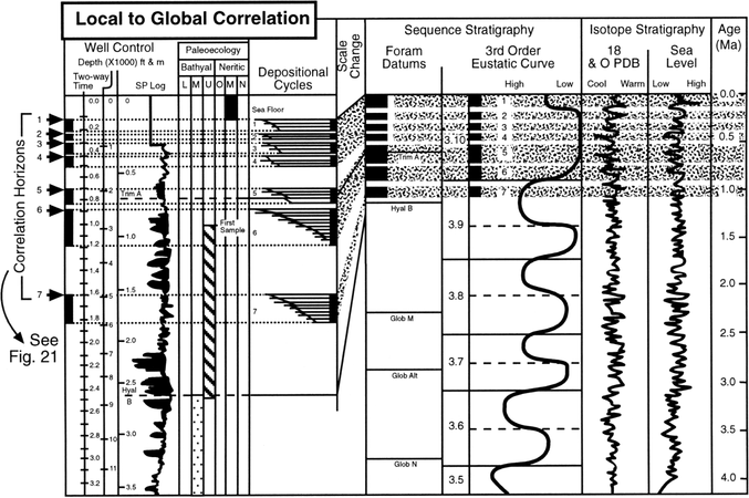
Figure 1 Correlation of the third-order eustatic curve of Haq et al.[1] and the oxygen isotope curve of Williams and Trainor[6] with seven prograding clinoform intervals from the High Island South Addition in the GOM basin. Copyright: Armentrout;[4] courtesy Gulf Coast SEPM and Geological Society of London.
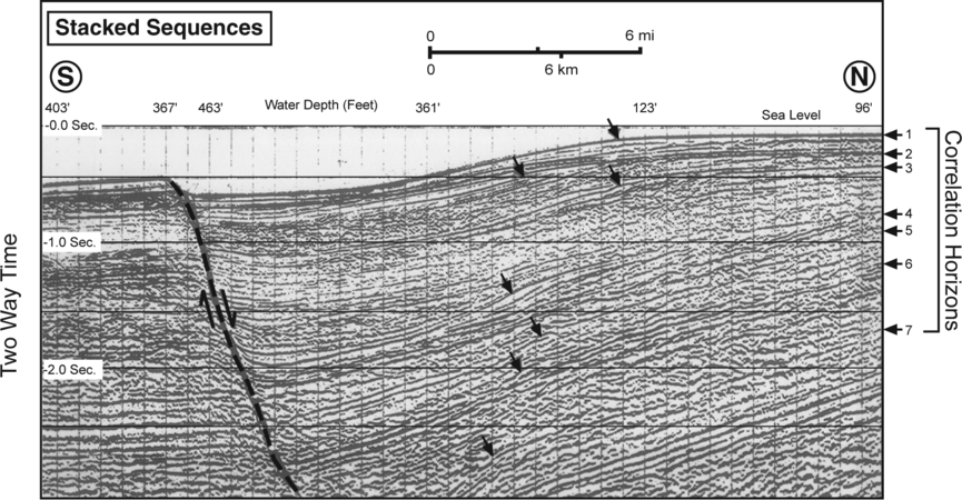
Figure 2 Seismic reflection profile. Copyright: Armentrout;[4] courtesy Gulf Coast SEPM and Geological Society of London.


Figure 1 shows the correlation of the third-order eustatic curve of Haq et al.[1] and the oxygen isotope curve of Williams and Trainor[6] with seven prograding clinoform intervals from the High Island South Addition in the GOM basin (see Figure 2). The correlations were established using the extinction events of the benthic foraminifera Hyalinea balthica (Hyal B) and Trimosina denticulata (Trim A) and the present-day sea floor as chronostratigraphic data. Six of the observed depositional cycles occur during the Tejas supersequence B 3.10 (0.8-0.0 Ma) third-order cycle of Haq et al.[1]). This correlation suggests that the local cycles are fourth-order depositional cycles with a duration of approximately 130,000 years each.[5]
The seven fourth-order cycles occur at approximately the same frequency as the oxygen isotope warm and cold cycles. The oxygen isotope cycles are interpreted as glacial-inter-glacial cycles corresponding with relative high- and lowstands of sea level.[6] The clinoforms generally correlate with trends in upward enrichment in isotope values, suggesting progradation during onset of glacial climates as a consequence of lowering sea level as continental ice formed.
See also
- Sea level cycle phase
- Sea level cycle phase and systems tracts
- Systems tracts identification
- Systems tracts and trap types
- Identifying sea level cycle phase with biostratigraphy
- Biofacies and changing sea level
- Constructing age model charts
- Superimposed sea level cycles
- Sequence stratigraphy
References
- ↑ 1.0 1.1 1.2 1.3 Haq, B., Hardenbol, J., Vail, P., R., 1988, Mesozoic and Cenozoic chronostratigraphy and cycles of sea-level change: SEPM Special Publication 42, p. 71–108.
- ↑ Miall, A., D., 1994, Paleocene 16: sequence stratigraphy and chronostratigraphy—problems of definition and precision in correlation, and their implications for global eustasy: Geoscience Canada, vol. 21, no. 1, p. 1–26.
- ↑ Armentrout, J., M., 1991, Paleontological constraints on depositional modeling: examples of integration of biostratigraphy and seismic stratigraphy, Pliocene–Pleistocene, Gulf of Mexico, in Weimer, P., Link, M., H., eds., Seismic Facies and Sedimentary Processes of Submarine Fans and Turbidite Systems: New York, Springer-Verlag, p. 137–170.
- ↑ 4.0 4.1 4.2 Armentrout, J., M., 1996, High-resolution sequence biostratigraphy: examples from the Gulf of Mexico Plio–Pleistocene, in Howell, J., Aiken, J., eds., High Resolution Sequence stratigraphy: Innovations and Applications: The Geological Society of London Special Publication 104, p. 65–86.
- ↑ 5.0 5.1 Mitchum, R., M., Jr., Van Wagoner, J., C., 1990, High-frequency sequences and eustatic cycles in the Gulf of Mexico basin: Proceedings, Gulf Coast Section SEPM 11th Annual Research conference, p. 257–267.
- ↑ 6.0 6.1 6.2 Williams, D., F., Trainor, D., M., 1987, Integrated chemical stratigraphy of deep-water frontier areas of the northern Gulf of Mexico: Proceedings, Gulf Coast Section SEPM 8th Annual Research conference, p. 151–158.
External links
| find literature about Sea level cycle order |