Difference between revisions of "Pc curves and saturation profiles"
Cwhitehurst (talk | contribs) |
Cwhitehurst (talk | contribs) m (added Category:Treatise Handbook 3 using HotCat) |
||
| (12 intermediate revisions by 3 users not shown) | |||
| Line 6: | Line 6: | ||
| part = Predicting the occurrence of oil and gas traps | | part = Predicting the occurrence of oil and gas traps | ||
| chapter = Predicting reservoir system quality and performance | | chapter = Predicting reservoir system quality and performance | ||
| − | | frompg = 9- | + | | frompg = 9-34 |
| − | | topg = 9- | + | | topg = 9-35 |
| author = Dan J. Hartmann, Edward A. Beaumont | | author = Dan J. Hartmann, Edward A. Beaumont | ||
| link = http://archives.datapages.com/data/specpubs/beaumont/ch09/ch09.htm | | link = http://archives.datapages.com/data/specpubs/beaumont/ch09/ch09.htm | ||
| Line 20: | Line 20: | ||
* The water–hydrocarbon saturation of a flow unit at different buoyancy pressures. | * The water–hydrocarbon saturation of a flow unit at different buoyancy pressures. | ||
| − | Placing flow units into structural cross | + | Placing flow units into [[Cross section#Structural cross section|structural cross section]]s shows their position with respect to the [[free water level]] and buoyancy pressure profile. Using the structure sections, saturation profiles can be made for each flow unit, their corresponding containers, and the reservoir as a whole. |
==Pore throat size and saturation profiles== | ==Pore throat size and saturation profiles== | ||
| − | [[file:predicting-reservoir-system-quality-and-performance_fig9-22.png|thumb|{{figure number|1}} | + | [[file:predicting-reservoir-system-quality-and-performance_fig9-22.png|300px|thumb|{{figure number|1}}Example reservoir cross section.]] |
| − | Water in the pore throats of rocks with macroporosity offers little capillary resistance to migrating hydrocarbons compared with the pore throats of rocks with microporosity. As a result, oil and gas migrate through a rock with macroporosity with minimal buoyancy pressure, i.e., hydrocarbon column. Macropore reservoirs have little or no saturation transition zone. | + | Water in the pore throats of rocks with macroporosity offers little capillary resistance to migrating hydrocarbons compared with the pore throats of rocks with microporosity. As a result, oil and gas migrate through a rock with macroporosity with minimal buoyancy pressure, i.e., [[hydrocarbon column]]. Macropore reservoirs have little or no saturation transition zone. |
| − | In rocks with microporosity, capillary forces hold water tightly to rock surfaces, decreasing the effective size of the already small pore throats. Therefore, a greater buoyancy pressure is required for oil or gas to migrate. Micropore reservoirs have longer saturation transition zones than | + | In rocks with microporosity, capillary forces hold water tightly to rock surfaces, decreasing the effective size of the already small pore throats. Therefore, a greater buoyancy pressure is required for oil or gas to migrate. Micropore reservoirs have longer saturation transition zones than macroporous or [[Wikipedia:Mesoporous material|mesoporous]] reservoirs; immobile water saturation is lower in macroporous rocks. |
| − | In the example reservoir cross section in [[:file:predicting-reservoir-system-quality-and-performance_fig9-22.png| | + | In the example reservoir [[cross section]] in [[:file:predicting-reservoir-system-quality-and-performance_fig9-22.png|Figure 1]], the rock in container 1 is mesoporous; the rock in container 2 is macroporous. Container 1 has a longer transition zone than container 2 because of this. Both containers have the same buoyancy pressure and free water level because the two containers are in pressure communication. |
==Pore throat size sorting== | ==Pore throat size sorting== | ||
| − | |||
| − | [[file:predicting-reservoir-system-quality-and-performance_fig9-23.png|thumb|{{figure number| | + | [[file:predicting-reservoir-system-quality-and-performance_fig9-23.png|300px|thumb|{{figure number|2}}Hypothetical examples of P<sub>c</sub> curves for rocks with varying pore throat size sorting.]] |
| + | |||
| + | The graph in [[:file:predicting-reservoir-system-quality-and-performance_fig9-23.png|Figure 2]] shows hypothetical examples of P<sub>c</sub> curves for rocks with varying pore throat size sorting. The [[Characterizing_rock_quality#What_is_r35.3F|r<sub>35</sub>]] value is the same for each sample; therefore, all three curves pass through the same point. The curves labeled A illustrate different pore throat size sorting. If the pore throats of the sample have a narrow range of sizes (i.e., are well sorted), the P<sub>c</sub> curve will be flat as the pressure in the mercury reaches the entry pressure for those pore throats. If the range of pore throat sizes is wide, the curve will steepen. | ||
==Making s<sub>w</sub> profiles from p<sub>c</sub> curves== | ==Making s<sub>w</sub> profiles from p<sub>c</sub> curves== | ||
If a P<sub>c</sub> curve is available, then a profile of S<sub>w</sub> can be approximated using information from the curve. To make an S<sub>w</sub> profile of a reservoir using a P<sub>c</sub> curve, use the table below. | If a P<sub>c</sub> curve is available, then a profile of S<sub>w</sub> can be approximated using information from the curve. To make an S<sub>w</sub> profile of a reservoir using a P<sub>c</sub> curve, use the table below. | ||
| − | + | # Convert pressure scale (Y-axis) to hydrocarbon column length ( ''h'' ), where h = P<sub>c</sub> × conversion factor (if conversion is unknown, use 0.7 for oil and 0.4 for gas). | |
| − | + | # Using the same scales, plot the curve next to a [[Cross section#Structural cross section|structure section]] showing the trap. Place the base of the curve at the free water level (see Figure 9-23). | |
| − | + | # Estimate S<sub>w</sub> for any point in the reservoir by reading the S<sub>w</sub> that corresponds to the depth. | |
| − | |||
| − | |||
| − | |||
| − | |||
| − | |||
| − | |||
| − | |||
| − | |||
| − | |||
| − | |||
| − | |||
==See also== | ==See also== | ||
| − | * [[ | + | * [[Pore-fluid interaction]] |
* [[Hydrocarbon expulsion, migration, and accumulation]] | * [[Hydrocarbon expulsion, migration, and accumulation]] | ||
* [[Characterizing rock quality]] | * [[Characterizing rock quality]] | ||
| Line 70: | Line 60: | ||
[[Category:Predicting the occurrence of oil and gas traps]] | [[Category:Predicting the occurrence of oil and gas traps]] | ||
[[Category:Predicting reservoir system quality and performance]] | [[Category:Predicting reservoir system quality and performance]] | ||
| + | [[Category:Treatise Handbook 3]] | ||
Latest revision as of 16:53, 4 April 2022
| Exploring for Oil and Gas Traps | |

| |
| Series | Treatise in Petroleum Geology |
|---|---|
| Part | Predicting the occurrence of oil and gas traps |
| Chapter | Predicting reservoir system quality and performance |
| Author | Dan J. Hartmann, Edward A. Beaumont |
| Link | Web page |
| Store | AAPG Store |
Water–hydrocarbon saturation profiles for a reservoir can be approximated using the capillary pressure (Pc) curves for the flow units it contains. The data in a Pc curve can be converted to give the following:
- An estimate of buoyancy pressures required to enter the pore throats of flow units.
- The radius of pore throats entered at a given buoyancy pressure.
- The water–hydrocarbon saturation of a flow unit at different buoyancy pressures.
Placing flow units into structural cross sections shows their position with respect to the free water level and buoyancy pressure profile. Using the structure sections, saturation profiles can be made for each flow unit, their corresponding containers, and the reservoir as a whole.
Pore throat size and saturation profiles
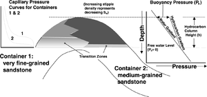
Water in the pore throats of rocks with macroporosity offers little capillary resistance to migrating hydrocarbons compared with the pore throats of rocks with microporosity. As a result, oil and gas migrate through a rock with macroporosity with minimal buoyancy pressure, i.e., hydrocarbon column. Macropore reservoirs have little or no saturation transition zone.
In rocks with microporosity, capillary forces hold water tightly to rock surfaces, decreasing the effective size of the already small pore throats. Therefore, a greater buoyancy pressure is required for oil or gas to migrate. Micropore reservoirs have longer saturation transition zones than macroporous or mesoporous reservoirs; immobile water saturation is lower in macroporous rocks.
In the example reservoir cross section in Figure 1, the rock in container 1 is mesoporous; the rock in container 2 is macroporous. Container 1 has a longer transition zone than container 2 because of this. Both containers have the same buoyancy pressure and free water level because the two containers are in pressure communication.
Pore throat size sorting
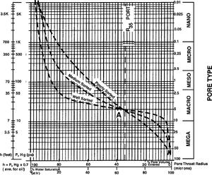
The graph in Figure 2 shows hypothetical examples of Pc curves for rocks with varying pore throat size sorting. The r35 value is the same for each sample; therefore, all three curves pass through the same point. The curves labeled A illustrate different pore throat size sorting. If the pore throats of the sample have a narrow range of sizes (i.e., are well sorted), the Pc curve will be flat as the pressure in the mercury reaches the entry pressure for those pore throats. If the range of pore throat sizes is wide, the curve will steepen.
Making sw profiles from pc curves
If a Pc curve is available, then a profile of Sw can be approximated using information from the curve. To make an Sw profile of a reservoir using a Pc curve, use the table below.
- Convert pressure scale (Y-axis) to hydrocarbon column length ( h ), where h = Pc × conversion factor (if conversion is unknown, use 0.7 for oil and 0.4 for gas).
- Using the same scales, plot the curve next to a structure section showing the trap. Place the base of the curve at the free water level (see Figure 9-23).
- Estimate Sw for any point in the reservoir by reading the Sw that corresponds to the depth.
See also
- Pore-fluid interaction
- Hydrocarbon expulsion, migration, and accumulation
- Characterizing rock quality
- Converting Pc curves to buoyancy, height, and pore throat radius
- What is permeability?
- Relative permeability and pore type

