Difference between revisions of "Water saturation distribution in a reservoir"
Cwhitehurst (talk | contribs) m (added Category:Treatise Handbook 3 using HotCat) |
|||
| (3 intermediate revisions by the same user not shown) | |||
| Line 6: | Line 6: | ||
| part = Predicting the occurrence of oil and gas traps | | part = Predicting the occurrence of oil and gas traps | ||
| chapter = Predicting reservoir system quality and performance | | chapter = Predicting reservoir system quality and performance | ||
| − | | frompg = 9- | + | | frompg = 9-65 |
| − | | topg = 9- | + | | topg = 9-67 |
| author = Dan J. Hartmann, Edward A. Beaumont | | author = Dan J. Hartmann, Edward A. Beaumont | ||
| link = http://archives.datapages.com/data/specpubs/beaumont/ch09/ch09.htm | | link = http://archives.datapages.com/data/specpubs/beaumont/ch09/ch09.htm | ||
| Line 18: | Line 18: | ||
==BVW== | ==BVW== | ||
<gallery mode=packed heights=250px widths=205px> | <gallery mode=packed heights=250px widths=205px> | ||
| − | file:predicting-reservoir-system-quality-and-performance_fig9-40.png|{{figure number|1}}How a Buckles plot relates to capillary pressure, fluid distribution, and fluid recovery in a reservoir. | + | file:predicting-reservoir-system-quality-and-performance_fig9-40.png|{{figure number|1}}How a [[Buckles plot]] relates to capillary pressure, fluid distribution, and fluid recovery in a reservoir. |
file:predicting-reservoir-system-quality-and-performance_fig9-41.png|{{figure number|2}}Hypothetical example of an S<sub>w</sub>–depth plot with estimated S<sub>w</sub> distribution curves for several flow units for a hydrocarbon-bearing zone in a well. | file:predicting-reservoir-system-quality-and-performance_fig9-41.png|{{figure number|2}}Hypothetical example of an S<sub>w</sub>–depth plot with estimated S<sub>w</sub> distribution curves for several flow units for a hydrocarbon-bearing zone in a well. | ||
file:predicting-reservoir-system-quality-and-performance_fig9-42.png|{{figure number|3}}Empirical ternary diagram for estimating height above free water, pore type (r<sub>35</sub>), and S<sub>w</sub> for a flow unit when the other two variables are known. | file:predicting-reservoir-system-quality-and-performance_fig9-42.png|{{figure number|3}}Empirical ternary diagram for estimating height above free water, pore type (r<sub>35</sub>), and S<sub>w</sub> for a flow unit when the other two variables are known. | ||
| Line 45: | Line 45: | ||
==Height–s<sub>w</sub>–pore type diagram== | ==Height–s<sub>w</sub>–pore type diagram== | ||
| − | The empirical ternary diagram in [[:file:predicting-reservoir-system-quality-and-performance_fig9-42.png|Figure 3]] is handy for estimating either height above free water, pore type ([[Characterizing_rock_quality#What_is_r35.3F|r<sub>35</sub>]]), or S<sub>w</sub> for a flow unit when the other two variables are known. For example, if S<sub>w</sub> for a flow unit is 20% and the pore type is macro with a port size of approximately 3μ, then the height above free water for the flow unit is approximately [[length::100 ft]]. Assumptions for the diagram include 30°API gravity oil, saline formation water, and a water-wet reservoir. | + | The empirical ternary diagram in [[:file:predicting-reservoir-system-quality-and-performance_fig9-42.png|Figure 3]] is handy for estimating either height above free water, pore type ([[Characterizing_rock_quality#What_is_r35.3F|r<sub>35</sub>]]), or S<sub>w</sub> for a flow unit when the other two variables are known. For example, if S<sub>w</sub> for a flow unit is 20% and the pore type is macro with a port size of approximately 3μ, then the height above free water for the flow unit is approximately [[length::100 ft]]. Assumptions for the diagram include 30°API [[gravity]] oil, saline formation water, and a water-wet reservoir. |
==See also== | ==See also== | ||
| Line 58: | Line 58: | ||
[[Category:Predicting the occurrence of oil and gas traps]] | [[Category:Predicting the occurrence of oil and gas traps]] | ||
[[Category:Predicting reservoir system quality and performance]] | [[Category:Predicting reservoir system quality and performance]] | ||
| + | [[Category:Treatise Handbook 3]] | ||
Latest revision as of 17:09, 5 April 2022
| Exploring for Oil and Gas Traps | |

| |
| Series | Treatise in Petroleum Geology |
|---|---|
| Part | Predicting the occurrence of oil and gas traps |
| Chapter | Predicting reservoir system quality and performance |
| Author | Dan J. Hartmann, Edward A. Beaumont |
| Link | Web page |
| Store | AAPG Store |
The distribution of water saturation (Sw) values within a reservoir depends on the height above free water, hydrocarbon type, pore throat-size distribution, and pore geometry. Mapping Sw distribution in a reservoir helps us predict trap boundaries.
BVW[edit]
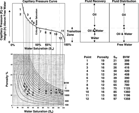
Figure 1 How a Buckles plot relates to capillary pressure, fluid distribution, and fluid recovery in a reservoir.
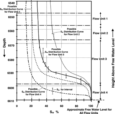
Figure 2 Hypothetical example of an Sw–depth plot with estimated Sw distribution curves for several flow units for a hydrocarbon-bearing zone in a well.
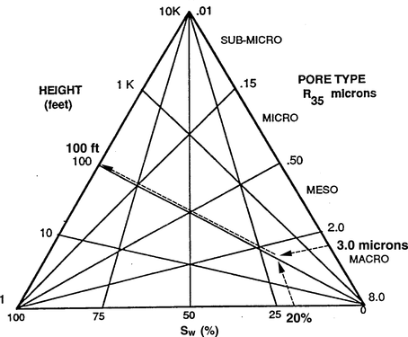
Figure 3 Empirical ternary diagram for estimating height above free water, pore type (r35), and Sw for a flow unit when the other two variables are known.


Bulk volume water (BVW) equals porosity (Φ) × Sw. In zones with the same pore type and geometry, BVW is a function of the height above the free water level. Above the transition zone, BVW is fairly constant. Below the transition zone, BVW is variable.
A Buckles plot is a plot of Sw vs. porosity. Contours of equal BVW are drawn on the plot.
- Points plot on a hyperbolic BVW line where the formation is near immobile water if the points come from a reservoir with consistent pore type and pore geometry.
- Points scatter on a Buckles plot where the formation falls below the top of the transition zone.
Figure 1 shows how a Buckles plot relates to capillary pressure, fluid distribution, and fluid recovery in a reservoir.
Limitations of BVW[edit]
BVW and Buckles plots can be confusing in interbedded lithologies or in areas where facies changes occur because of changing pore types.
Sw–depth plots[edit]
These illustrate how Sw varies within a hydrocarbon-bearing zone. Variations reflect different pore types and/or height above free water. An Sw–depth plot can be used to delineate three things:
- Transition and waste zones
- Flow units
- Containers
Individual plots can be prepared for wells along dip and strike and correlated to show Sw changes across a reservoir or field. Figure 2 is a hypothetical example of an Sw–depth plot with estimated Sw distribution curves for several flow units for a hydrocarbon-bearing zone in a well.
Height–sw–pore type diagram[edit]
The empirical ternary diagram in Figure 3 is handy for estimating either height above free water, pore type (r35), or Sw for a flow unit when the other two variables are known. For example, if Sw for a flow unit is 20% and the pore type is macro with a port size of approximately 3μ, then the height above free water for the flow unit is approximately length::100 ft. Assumptions for the diagram include 30°API gravity oil, saline formation water, and a water-wet reservoir.
See also[edit]
External links[edit]
| find literature about Water saturation distribution in a reservoir |